Day 4 - $\LaTeX$ and Quarto

Suggested citation: Parushya. (2024). “Employing the Olympic Shooter Meme for Quarto Adoption”. In Hashem and Parushya (Eds.), *Math Camp 2024*

Software Session

WTH is $\LaTeX$?
Why Quarto?
Basics

Yaml
Markdown text
Code Chunks

Practice

WTH is $\LaTeX$?

$\LaTeX$ (pronounced “LAY-tek” or “LAH-Tek) is a typesetting tool for preparing high-quality professional documents. It is the preferred typesetting tool used in high-end scientific documentation task. Essentially, it allows you better control over how your document look like, has enhanced capabilities to write technical specifications (Maths, stats, proofs, etc.), and produces readily editable back-end documents.

It is not a word-processing tool. It is a simple tool without too many priors about how the document should look like.

In academic world there are definite advantages to learning and being comfortable with $\LaTeX$. That would require regular use and best time to start doing that would be today (or at least next week!).

There are many interfaces that allow you to work with $\LaTeX$. Overleaf is a widely used online platform and Texmaker is a popular offline application.

However, RStudio has in-built capability to double as a $\LaTeX$ editor. Previously RMarkdown and now Quarto are those capabilities that you can harness to achieve professional and beautifully typeset documents.

Think of writing an equation like:
\[ Violence_{i,j} = \beta_0 + \beta_1EthnicFractionalization_i + \gamma_j + \epsilon_i \] In Latex, using quarto, you have to write something like the following:

$Violence_{i,j} = \\beta_0 + \\beta_1EthnicFractionalization_i + \\gamma_j + \\epsilon_i$

For a single line of text we encapsulate code by $ sign.

For multi-line code we use $$.

Quarto

Quarto is a literate statistical programming tool. Literate statistical programming, as Donald Knuth (1984) defines, is a way to write programs that focuses on explaining to human readers what we want the computers to do, rather than just instructing the computers to do so.

Quarto can include code from not just R, but also Python, Julia, Stata and many other languages/tools.

Quarto allows you to truly include the good coding guidelines that we discussed on day 1. It provides you with capability to write code using R, write text that is part of any professional communication, and include mathematical symbols and equations in a well typeset format. Essentially, it allows you to work on a manuscript with data analysis at one place.

Here is some cool stuff that you can do with quarto.

Exercise 1

Open a new quarto document by File > New File > Quarto Document.
Use Render button on top on scripts panel to save and get a .pdf output.

Basics

A Quarto document is saved as a .qmd file. You can edit this file in two ways: Programmatically by being in source button and visually by choosing the Visual button, both button on top left corner of the .qmd window. More details about workign with Quarto can be found on the quarto website here.

There are three building blocks in a .qmd file:

YAML

Short for Yet-Another-Markup-Languge

This is the part we see sandwiched between two --- at the strat of .qmd file. Here we define different global settings for the particular document.

Currently, we see

---
title: "Untitled"
format: html
---

We can add many more options here to modify the details to appear at the start of the document. Here’s an example from quarto reference site

  ---
  title: "Toward a Unified Theory of High-Energy Metaphysics: Silly String Theory"
  date: 2008-02-29
  author:
    - name: Josiah Carberry
      id: jc
      orcid: 0000-0002-1825-0097
      email: josiah@psychoceramics.org
      affiliation: 
        - name: Brown University
          city: Providence
          state: RI
          url: www.brown.edu
  abstract: > 
    The characteristic theme of the works of Stone is 
    the bridge between culture and society. ...
  keywords:
    - Metaphysics
    - String Theory
  license: "CC BY"
  copyright: 
    holder: Josiah Carberry
    year: 2008
  citation: 
    container-title: Journal of Psychoceramics
    volume: 1
    issue: 1
    doi: 10.5555/12345678
  funding: "The author received no specific funding for this work."
  ---

Or, global settings for different formats of outputs like

---
title: "My Document"
format: 
  html:
    fig-width: 8
    fig-height: 6
  pdf:
    fig-width: 7
    fig-height: 5
---

Code Chunks

One of the fascinating features about quarto is that you can write code to anlayse data and regular text in the same document.

You can start a new R code chunk by pressing cmd + option + I or ctrl + alt + I.

You can also do this with the Insert button icon in the editor toolbar or by manually typing the chunk delimiters ```{r} and ```.

Try to use the keyboard shortcut more often as it will save you a ton of time later.

R code chunks are surrounded by ```{r} and ```.

You can run each code chunk by clicking the Run icon (it looks like a play button at the top of the chunk), or by pressing Cmd/Ctrl + Shift + Enter.

#| eval: true # Do evaluate this chunk
#| echo: true # Do show this chunk in the final rendered document
#| output: true # Do show the output / results of this chunk in the rendered document

print("Dont run this code")

RStudio executes the code and displays the results below the code.

If you don’t like seeing your plots and output in your document and would rather make use of RStudio’s Console and Plot panes, you can click on the gear icon next to “Render” and switch to “Chunk Output in Console”.

A chunk should be relatively self-contained, and focused around a single task.

Exercise

Add a code chunk at the bottom of the .qmd file you created.
Add some simple mathematical operations from the exercises on Day 2 in the code chunk.
Run the code chunk separately, and then the whole file by pressing Render button from the top.

Code chunk options are included in a special comment at the top of the block (lines at the top prefaced with #| are considered options). More on code chunk options here

Options available for customizing output include:

Option	Description
`eval`	Evaluate the code chunk (if `false`, just echos the code into the output).
`echo`	Include the source code in output
`output`	Include the results of executing the code in the output (`true`, `false`, or `asis` to indicate that the output is raw markdown and should not have any of Quarto’s standard enclosing markdown).
`warning`	Include warnings in the output.
`error`	Include errors in the output (note that this implies that errors executing code will not halt processing of the document).
`include`	Catch all for preventing any output (code or results) from being included (e.g. `include: false` suppresses all output from the code block).

You can also add these options as global options in the YAML by writing them under execute option like:

---
execute: 
  echo: true
  inlcude: false
---

The following table summarizes which types of output each option suppresses:¹

Option	Run code	Show code	Output	Plots	Messages	Warnings
`eval: false`	X		X	X	X	X
`include: false`		X	X	X	X	X
`echo: false`		X
`results: hide`			X
`fig-show: hide`				X
`message: false`					X
`warning: false`						X

Inline code

We can also embed R code into a Quarto document: directly into the text, with: ```{r} <code> ```.

For example: ```{r} (2+2)```.

Markdown Text

Markdown text is like any other text just with some special considerations.

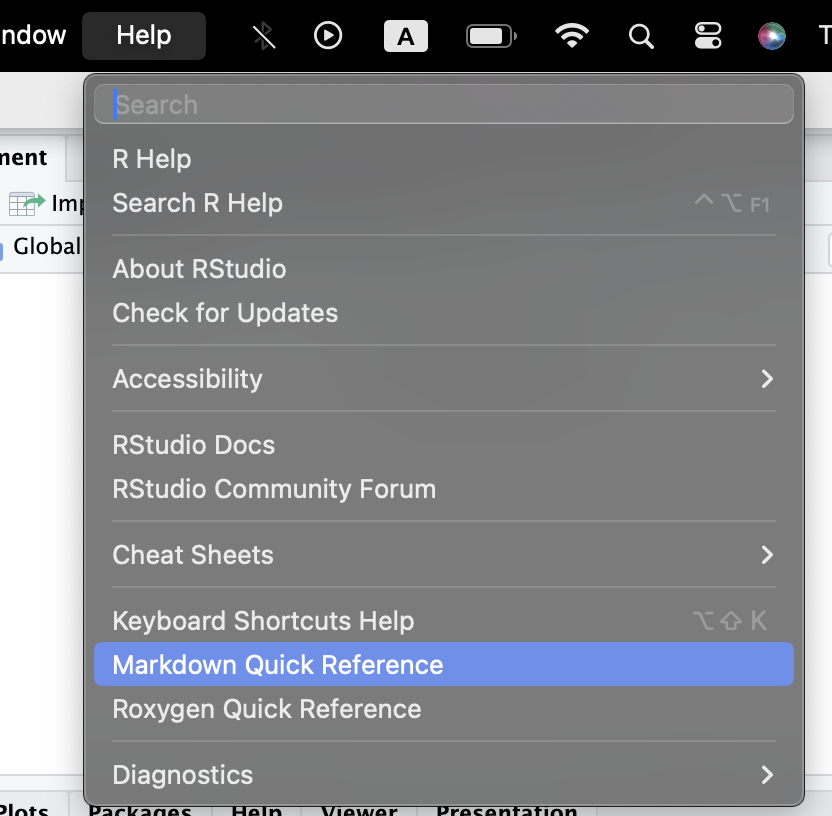
You can see the help section from R to see some of the basic formatting tips.

These are some of the regularly used formatting options in RMarkdown/Quarto Titles and subtitles ————————————————————

# Title 1

## Title 2

### Title 3


Text formatting 
------------------------------------------------------------

*italic*  

**bold**   

`code`

Lists
------------------------------------------------------------

* Bulleted list item 1
* Item 2
  * Item 2a
  * Item 2b

1. Item 1
2. Item 2

Links and images
------------------------------------------------------------

Practice

Let’s try all that we learnt

Exercise

Delete the existing code in the .qmd file that we created today.
Add some simple mathematical operations from the exercises on Day 2 in the code chunk (like the previous exercise). Now, in the chunk set the options differently. You could play with different options that we learnt above and their values. Use <TAB> button to see different values that you can provide to chunk options.

```{r}
#| echo: true
#| output: asis

1 + 1
```

[1] 2

Add two separate R chunks. First, load the VDEM data as we did yesterday in one. Second, to filter data to year 2021 and select the variables - year, country_name, v2x_libdem, e_gdppc, e_pop.

```{r}
#| echo: false 
#| message: false
#| warning: false

# Loading packages
library(tidyverse) # For tidyverse
library(janitor) # For Janitor

# Loading Dataset
vdem_df <- readRDS("Datasets-mathcamp/V-Dem-CY-Full+Others-v12.rds") %>% 
clean_names() 

# ` %>% ` is the piping operator from tidyverse universe

# `clean_names` cleans the names of columns and standardizes them | from Janitor package
```

```{r}
#| echo: false  # Toggle with options as well the paramters like true/false etc
#| message: false
#| warning: false
vdem_2021 <- vdem_df %>% 
  filter(year == 2021) %>%  # To filter values according to one variable
  select(year, country_name, v2x_libdem, e_gdppc, e_pop) # To select particular variables
```

Run the following code to plot v2x_libdem on x-axis and e_gdppc on y-axis.

```{r}
#| echo: false  # Toggle with options as well the paramters like true/false etc
#| message: false
#| warning: false

ggplot( data = vdem_df, aes( x = v2x_libdem, y = e_gdppc)) +
geom_point()

```

Add a least-squares/ linear regression line to the plot.

```{r}
#| echo: false  # Toggle with options as well the paramters like true/false etc
#| message: false
#| warning: false

ggplot( data = vdem_df, aes( x = v2x_libdem, y = e_gdppc)) +
geom_point( alpha = 0.5) +
geom_smooth(method = "lm")
```

Tasks 3, 4 and 5 use ggplot which is a part of tidyverse. Follow the tidyverse book from Day 1 for understanding them well.

Find out what the variables v2x_libdem and e_gdppc mean from the VDem Codebook here. Write the details of the variable in the markdown text area of quarto explaining these variables.
We added a least squares best fit line in the second plot. Write a basic equation in LaTex that looks like this:

Model Equation
Model Latex Code

$LiberalDemocracy_i = \alpha + \beta_1GDPpc_i + epislon_i$

Render the whole document into a .pdf with your name in the YAML and today’s date. You may use the following YAML with modifications.

---
title: My First Latex Document
subtitle: Prepared for Math Camp 2024
author: <Your Name>
date: today
format:
  pdf:
    highlight-style: kate
    citation_package: natbib
  docx: default
always_allow_html: true
geometry: margin=1.2in
fontsize: 12pt
linestretch: 1.5
linkcolor: blue
toc: true
link-citations: true
editor_options: 
  chunk_output_type: console
execute: 
  fig-height: 6
  fig-width: 8.5
  fig-pos: "!t"
keep_tex: true
whitespace: small
---

If you think your thought is not making sense, write it in $\LaTeX$,

It will at least not make sense in a beautiful way.

-Buddha (500 B.C.E.)

Additonal Links

Quarto Official Guide

Quarto R for datascience

Quarto with RStudio

$\LaTeX$

Follow these instructions to install library(tinytex).

Intro to $\LaTeX$ in Markdown

This section is copied from R4DS book ↩︎

Day 4 - \(\LaTeX\) and Quarto

Software Session

WTH is \(\LaTeX\)?

Quarto

Basics

YAML

Code Chunks

Inline code

Markdown Text

Practice

Additonal Links

\(\LaTeX\)