# Install if needed (run once):
# install.packages(c("tidyverse"))

library(tidyverse) # loads ggplot2, dplyr, tidyr, readr, tibble, stringr, forcats, purrrDay 5 - R-eady to be Deployed!

By the end of today, you will be able to:
- Write conditional logic with
if,if...else, ladderedelse if, and nested conditionals. - Compute descriptive statistics and group-wise summaries using base R (
aggregate(),by(),table(),xtabs()). - Perform fast, readable data wrangling with dplyr:
select(),filter(),mutate(),arrange(),summarise(),group_by(),across(),distinct(), and basic joins. - Build layered visualizations with ggplot2 (scatter, histograms, density, box/violin/jitter, lines, bars, faceting, and annotations).
Data used:
mpg,economics(bundled with ggplot2).
Setup
Start by creating a new qmd file, like we did yesterday. Write/paste all the code from today in the same file so that we can render at the end.
```{r}
# Quick peek at the data we'll use
head(mpg)
str(mpg)
```
Conditionals in Base R
Conditional statements let your code make decisions.
Comparison operators (what they do)
==,!=: test equality / inequality (return TRUE/FALSE).>,>=,<,<=: numeric comparisons.&&,||: element-wise logic on single TRUE/FALSE values (short-circuit). Use&/|for vectorized logic.!: logical negation.
```{r}
x <- 10
y <- 20

x == y     # FALSE
x != y     # TRUE
x > 0      # TRUE
x >= 10    # TRUE
x < y      # TRUE
x <= y     # TRUE
```
if
- Runs a code block only if the condition is TRUE.
```{r}
if (x > 0) {
  print("x is a positive number")
}
```
if ... else
- Chooses one of two paths.
```{r}
if (x > y) {
  print("x is greater than y")
} else {
  print("y is greater than or equal to x")
}
```
Laddered else if
- Chains multiple mutually exclusive tests.
```{r}
x <- y
if (x > y) {
  print("x is greater than y")
} else if (y > x) {
  print("y is greater than x")
} else {
  print("x and y are equal")
}
```
Nested if
- Scope one decision inside another.
```{r}
x <- 20; y <- 10; z <- -30
if (x > y) {
  print("x is greater than y")
  if (x > z) {
    print("x is greater than y and z")
  }
}
```
Multiple conditions and the difference between &/| vs &&/||
```{r}
# For single TRUE/FALSE (first element only): &&, ||
if (x > y && x > z) {
  print("x is greater than both y and z")
}

# Vectorized comparisons across all elements: &, |
c(1,2,3) > 2 & c(10,20,30) > 15
```
Exercise
Write an if...else if...else ladder that prints "small", "medium", or "large" depending on the value of n relative to 10 and 100.
Descriptive Statistics & Aggregation (Base R)
Summarize the mpg dataset to understand central tendency, spread, and relationships.
Central tendency
mean(x): arithmetic average (sensitive to outliers).median(x): middle value (robust to outliers).
```{r}
mean(mpg$displ)
median(mpg$displ)

# Note: base R's mode() returns the storage mode, not the statistical mode.
mode(mpg$displ)
```
Spread & quantiles
var(x),sd(x): variance and SD.quantile(x, p): p-th quantile (e.g., 0.25 = Q1).IQR(x): Q3 - Q1.range(x),min(x),max(x).
```{r}
var(mpg$cty)
sd(mpg$cty)

quantile(mpg$cty, c(0.25, 0.75))
IQR(mpg$cty)

min(mpg$cty); max(mpg$cty)
range(mpg$cty)
```
Categorical summaries
table(x): counts by category.unique(x): distinct values.
```{r}
table(mpg$drv)
unique(mpg$cyl)
```
Group-wise means (manual vs. aggregate())
aggregate(y ~ g, FUN, data): summary of y by groups g.subset =lets you compute summaries on filtered rows.
```{r}
# Manual subsetting (repetitive)
mean(mpg$cty[mpg$cyl == 4])
mean(mpg$cty[mpg$cyl == 6])
mean(mpg$cty[mpg$cyl == 8])

# Using aggregate(): dv ~ iv
aggregate(cty ~ cyl, FUN = mean, data = mpg)

# Subset argument
aggregate(cty ~ cyl,
          FUN = mean,
          subset = cty < 15,
          data = mpg)
```
Quick summaries (summary(), by())
summary(df)gives per-column summaries.by(df, group, summary)appliessummary()within each group.
```{r}
summary(mpg)
summary(mpg$displ)

by(mpg, mpg$cyl, summary)
```
Contingency tables & proportions (table(), xtabs(), prop.table())
xtabs(~ a + b): formula interface for contingency tables.prop.table(tab, margin): convert counts to proportions (by rows1or columns2).
```{r}
# Counts
table(mpg$cyl, mpg$year)
xtabs(~ mpg$cyl + mpg$year)

# Relative frequencies
prop.table(table(mpg$year, mpg$class))
prop.table(table(mpg$year, mpg$class), 1)          # by row
round(prop.table(table(mpg$year, mpg$class), 2), 2) # by column (rounded)
round(prop.table(table(mpg$year, mpg$class), 2), 2) * 100
```
Mosaic plot
```{r}
mosaicplot(table(mpg$year, mpg$class),
           color = TRUE,
           xlab = "Year",
           ylab = "Class")
```
Exercise
Compute the median highway mileage (hwy) by number of cylinders (cyl) with aggregate(). Compare it to the corresponding boxplots in Section 4.6.
Data Wrangling with dplyr (Pipes, select, filter, mutate, summarise, joins)
The dplyr verbs make data manipulation fast and expressive. They work best with the pipe |> (base R) or %>% (magrittr). We’ll use |> here.
dplyr is a part of tidyverse universe. Tidyverse is an opiniated approach to data handling. What this means is that the packages and practices in this approach presuppose a particular format of data. The data either needs to be in the particular format or be transformed to one, for this approach to work efficiently. In practice, it is quite intuitive and simple.
There are three interrelated rules of tidy data are:
1- Each variable must have its own column.
2- Each observation must have its own row.
3- Each value must have its own cell.
You can read more about tidy data here.
Pipes
# Without pipe
head(arrange(select(mpg, manufacturer, model, hwy), desc(hwy)), 5)

# With pipe (clearer)
mpg |>
  select(manufacturer, model, hwy) |>
  arrange(desc(hwy)) |>
  head(5)
# A tibble: 5 × 3
manufacturer model hwy
<chr> <chr> <int>
1 volkswagen jetta 44
2 volkswagen new beetle 44
3 volkswagen new beetle 41
4 toyota corolla 37
5 honda civic 36# A tibble: 5 × 3
manufacturer model hwy
<chr> <chr> <int>
1 volkswagen jetta 44
2 volkswagen new beetle 44
3 volkswagen new beetle 41
4 toyota corolla 37
5 honda civic 36select() (choose columns)
mpg |>
  select(manufacturer, model, hwy)

mpg |>
  select(starts_with("d")) |>
  head(3)

# Rename while selecting
mpg |>
  select(make = manufacturer, model, hwy) |>
  head(3)

# Move columns around
mpg |>
  relocate(hwy, .before = displ) |>
  head(3)
# A tibble: 234 × 3
manufacturer model hwy
<chr> <chr> <int>
1 audi a4 29
2 audi a4 29
3 audi a4 31
4 audi a4 30
5 audi a4 26
6 audi a4 26
7 audi a4 27
8 audi a4 quattro 26
9 audi a4 quattro 25
10 audi a4 quattro 28
# ℹ 224 more rows# A tibble: 3 × 2
displ drv
<dbl> <chr>
1 1.8 f
2 1.8 f
3 2 f # A tibble: 3 × 3
make model hwy
<chr> <chr> <int>
1 audi a4 29
2 audi a4 29
3 audi a4 31# A tibble: 3 × 11
manufacturer model hwy displ year cyl trans drv cty fl class
<chr> <chr> <int> <dbl> <int> <int> <chr> <chr> <int> <chr> <chr>
1 audi a4 29 1.8 1999 4 auto(l5) f 18 p compa…
2 audi a4 29 1.8 1999 4 manual(m5) f 21 p compa…
3 audi a4 31 2 2008 4 manual(m6) f 20 p compa…filter() (keep rows)
mpg |>
  filter(class == "suv", hwy >= 20) |>
  head(5)

mpg |>
  filter(manufacturer %in% c("toyota", "honda")) |>
  count(manufacturer)
# A tibble: 5 × 11
manufacturer model displ year cyl trans drv cty hwy fl class
<chr> <chr> <dbl> <int> <int> <chr> <chr> <int> <int> <chr> <chr>
1 chevrolet c1500 subu… 5.3 2008 8 auto… r 14 20 r suv
2 chevrolet c1500 subu… 5.3 2008 8 auto… r 14 20 r suv
3 jeep grand cher… 3 2008 6 auto… 4 17 22 d suv
4 jeep grand cher… 4 1999 6 auto… 4 15 20 r suv
5 nissan pathfinder… 4 2008 6 auto… 4 14 20 p suv # A tibble: 2 × 2
manufacturer n
<chr> <int>
1 honda 9
2 toyota 34mutate() (create/modify columns)
mpg |>
  mutate(
    hwy_kmpl = hwy * 0.425144,           # convert mpg to km/L (approx)
    efficiency = case_when(
      hwy >= 30 ~ "high",
      hwy >= 20 ~ "medium",
      TRUE ~ "low"
    )
  ) |>
  select(manufacturer, model, hwy, hwy_kmpl, efficiency) |>
  head(6)
# A tibble: 6 × 5
manufacturer model hwy hwy_kmpl efficiency
<chr> <chr> <int> <dbl> <chr>
1 audi a4 29 12.3 medium
2 audi a4 29 12.3 medium
3 audi a4 31 13.2 high
4 audi a4 30 12.8 high
5 audi a4 26 11.1 medium
6 audi a4 26 11.1 medium arrange() (sort rows)
mpg |>
  arrange(manufacturer, desc(hwy)) |>
  head(6)
# A tibble: 6 × 11
manufacturer model displ year cyl trans drv cty hwy fl class
<chr> <chr> <dbl> <int> <int> <chr> <chr> <int> <int> <chr> <chr>
1 audi a4 2 2008 4 manua… f 20 31 p comp…
2 audi a4 2 2008 4 auto(… f 21 30 p comp…
3 audi a4 1.8 1999 4 auto(… f 18 29 p comp…
4 audi a4 1.8 1999 4 manua… f 21 29 p comp…
5 audi a4 quattro 2 2008 4 manua… 4 20 28 p comp…
6 audi a4 3.1 2008 6 auto(… f 18 27 p comp…group_by() + summarise() (grouped summaries)
mpg |>
  group_by(cyl) |>
  summarise(
    mean_cty = mean(cty),
    median_hwy = median(hwy),
    n = dplyr::n()
  )

mpg |>
  group_by(drv) |>
  summarise(across(c(cty, hwy), list(mean = mean, sd = sd)))
# A tibble: 4 × 4
cyl mean_cty median_hwy n
<int> <dbl> <dbl> <int>
1 4 21.0 29 81
2 5 20.5 29 4
3 6 16.2 24 79
4 8 12.6 17 70# A tibble: 3 × 5
drv cty_mean cty_sd hwy_mean hwy_sd
<chr> <dbl> <dbl> <dbl> <dbl>
1 4 14.3 2.87 19.2 4.08
2 f 20.0 3.63 28.2 4.21
3 r 14.1 2.22 21 3.66distinct(), slice(), sampling
# Unique combinations of columns
mpg |>
  distinct(manufacturer, class) |>
  head(10)

# Take specific rows by position
mpg |>
  slice(1:5)

# Random samples
set.seed(123)
mpg |>
  slice_sample(n = 5)
# A tibble: 10 × 2
manufacturer class
<chr> <chr>
1 audi compact
2 audi midsize
3 chevrolet suv
4 chevrolet 2seater
5 chevrolet midsize
6 dodge minivan
7 dodge pickup
8 dodge suv
9 ford suv
10 ford pickup # A tibble: 5 × 11
manufacturer model displ year cyl trans drv cty hwy fl class
<chr> <chr> <dbl> <int> <int> <chr> <chr> <int> <int> <chr> <chr>
1 audi a4 1.8 1999 4 auto(l5) f 18 29 p compa…
2 audi a4 1.8 1999 4 manual(m5) f 21 29 p compa…
3 audi a4 2 2008 4 manual(m6) f 20 31 p compa…
4 audi a4 2 2008 4 auto(av) f 21 30 p compa…
5 audi a4 2.8 1999 6 auto(l5) f 16 26 p compa…# A tibble: 5 × 11
manufacturer model displ year cyl trans drv cty hwy fl class
<chr> <chr> <dbl> <int> <int> <chr> <chr> <int> <int> <chr> <chr>
1 pontiac grand prix 5.3 2008 8 auto… f 16 25 p mids…
2 toyota toyota tac… 4 2008 6 auto… 4 16 20 r pick…
3 toyota 4runner 4wd 4.7 2008 8 auto… 4 14 17 r suv
4 audi a4 quattro 3.1 2008 6 auto… 4 17 25 p comp…
5 toyota corolla 1.8 1999 4 auto… f 24 33 r comp…Joins (combine tables by keys)
a <- tibble(id = c(1,2,3), val = c("A","B","C"))
b <- tibble(id = c(2,3,4), note = c("two","three","four"))

left_join(a, b, by = "id")
inner_join(a, b, by = "id")
full_join(a, b, by = "id")
anti_join(a, b, by = "id")  # rows in a without matches in b
semi_join(a, b, by = "id")  # rows in a that have a match in b
# A tibble: 3 × 3
id val note
<dbl> <chr> <chr>
1 1 A <NA>
2 2 B two
3 3 C three# A tibble: 2 × 3
id val note
<dbl> <chr> <chr>
1 2 B two
2 3 C three# A tibble: 4 × 3
id val note
<dbl> <chr> <chr>
1 1 A <NA>
2 2 B two
3 3 C three
4 4 <NA> four # A tibble: 1 × 2
id val
<dbl> <chr>
1 1 A # A tibble: 2 × 2
id val
<dbl> <chr>
1 2 B
2 3 C Reshaping with tidyr (bonus)
# Wide -> Long
wide <- tibble(id = 1:3, y_2020 = c(1,2,3), y_2021 = c(4,5,6))
long <- wide |>
  pivot_longer(starts_with("y_"), names_to = "year", values_to = "y")
long

# Long -> Wide
long |>
  pivot_wider(names_from = year, values_from = y)
# A tibble: 6 × 3
id year y
<int> <chr> <dbl>
1 1 y_2020 1
2 1 y_2021 4
3 2 y_2020 2
4 2 y_2021 5
5 3 y_2020 3
6 3 y_2021 6# A tibble: 3 × 3
id y_2020 y_2021
<int> <dbl> <dbl>
1 1 1 4
2 2 2 5
3 3 3 6
Quick Cheatsheet
- Columns:
select(),rename(),relocate() - Rows:
filter(),arrange(),slice() - New columns:
mutate(),if_else(),case_when() - Groups:
group_by(),summarise(),across() - Uniques & counts:
distinct(),count() - Joins:
left_join(),inner_join(),full_join(),anti_join(),semi_join() - Reshape:
pivot_longer(),pivot_wider()
Grammar of Graphics with ggplot2
ggplot is the R functional form of the Grammar of Graphics
But what does it mean?
The Grammar of Graphics was introduced to describe the deep structure underlying statistical graphics. Wilkinson (2005) formalized the idea of what a “statistical graphic” is; Wickham (2010) adapted that grammar into a layered system in R. In short, a statistical plot maps data to aesthetic attributes (e.g., colour, shape, size) of geometric objects (e.g., points, lines, bars), may include statistical transformations, is drawn on a coordinate system, and can be faceted to repeat the same plot over subsets of the data. It’s the combination of these independent components that makes a graphic.
ggplot2 is built on the idea: any plot can be expressed from the same set of components—a dataset, a coordinate system, and geoms (visual marks). The key to understanding ggplot2 is thinking in layers, much like stacked layers in image editors such as Photoshop/Illustrator/Inkscape.
The guiding principle in ggplot2 is to build from foundational components (data, global mappings) to specific components (geoms, stats, scales, guides), connecting layers with +. Think of each layer as placed on the same canvas; together they compose the plot. The general structure is:
ggplot(data = <DATA>, mapping = aes(<X>, <Y>, <global aesthetics>)) +
  geom_<TYPE>(aes(<layer-specific aesthetics>), <layer options>) +
  stat_<TRANSFORM>(...) +
  scale_<...>(...) +
  coord_<...>(...) +
  facet_<...>(...) +
  labs(title = "...", subtitle = "...", x = "...", y = "...") +
  theme(...)
The ggplot2 package builds plots by layering components: data, aesthetic mappings, geoms, statistics, scales, coordinates, and facets.
You can read more about ggplot here.
First plot
ggplot(mpg, aes(x = displ, y = hwy)) +
  geom_point()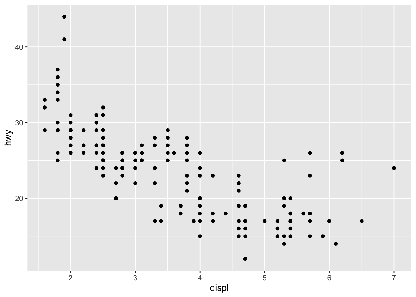
Compare to base R:
plot(x = mpg$displ, y = mpg$hwy)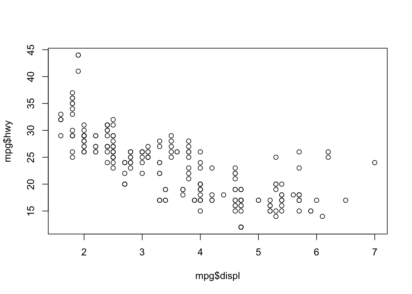
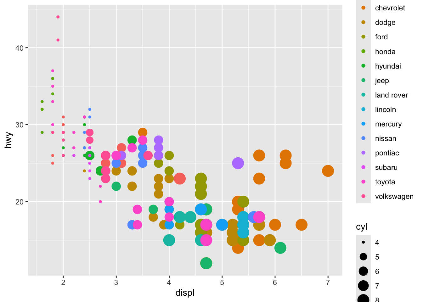
Aesthetics: colour, size, shape, alpha
ggplot(mpg, aes(displ, hwy, colour = manufacturer)) + geom_point()
ggplot(mpg, aes(displ, hwy, colour = manufacturer, size = cyl)) + geom_point()
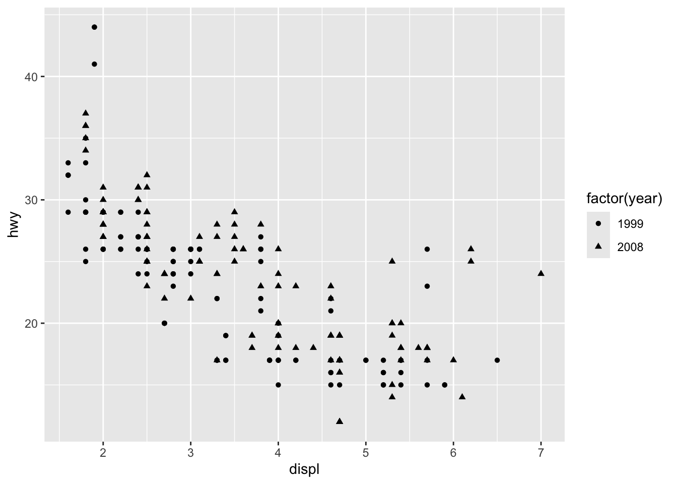
ggplot(mpg, aes(displ, hwy, shape = factor(year))) + geom_point()
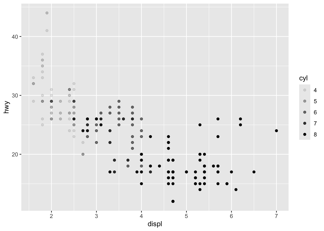
ggplot(mpg, aes(displ, hwy, alpha = cyl)) + geom_point()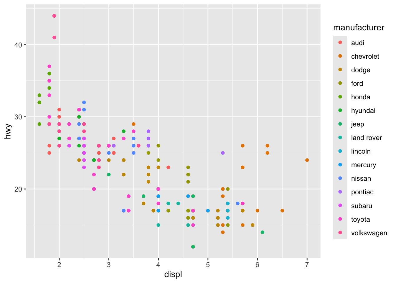
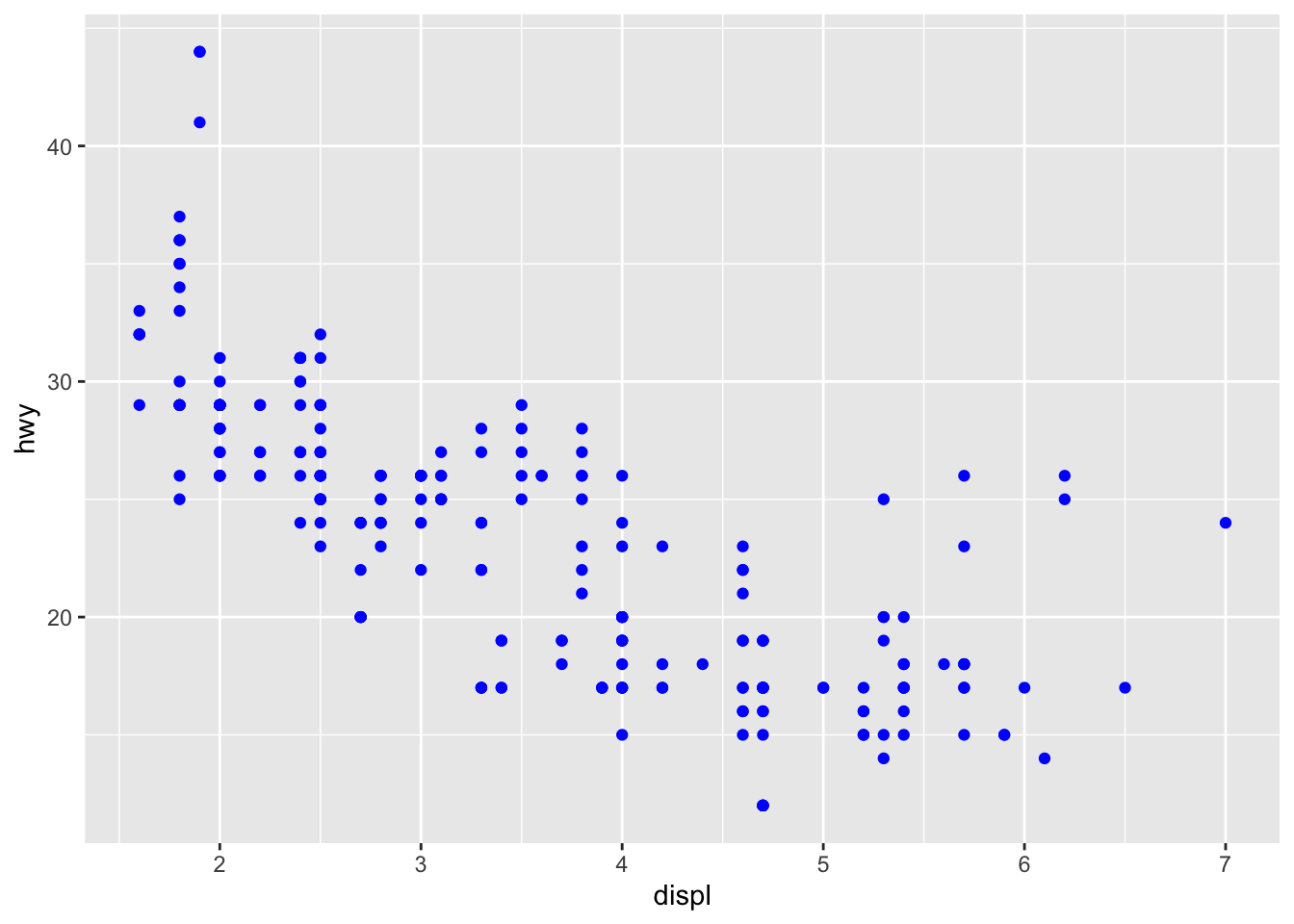
Fixed aesthetics (outside aes()):
ggplot(mpg, aes(displ, hwy)) + geom_point(aes(colour = "blue"))
ggplot(mpg, aes(displ, hwy)) + geom_point(colour = "blue")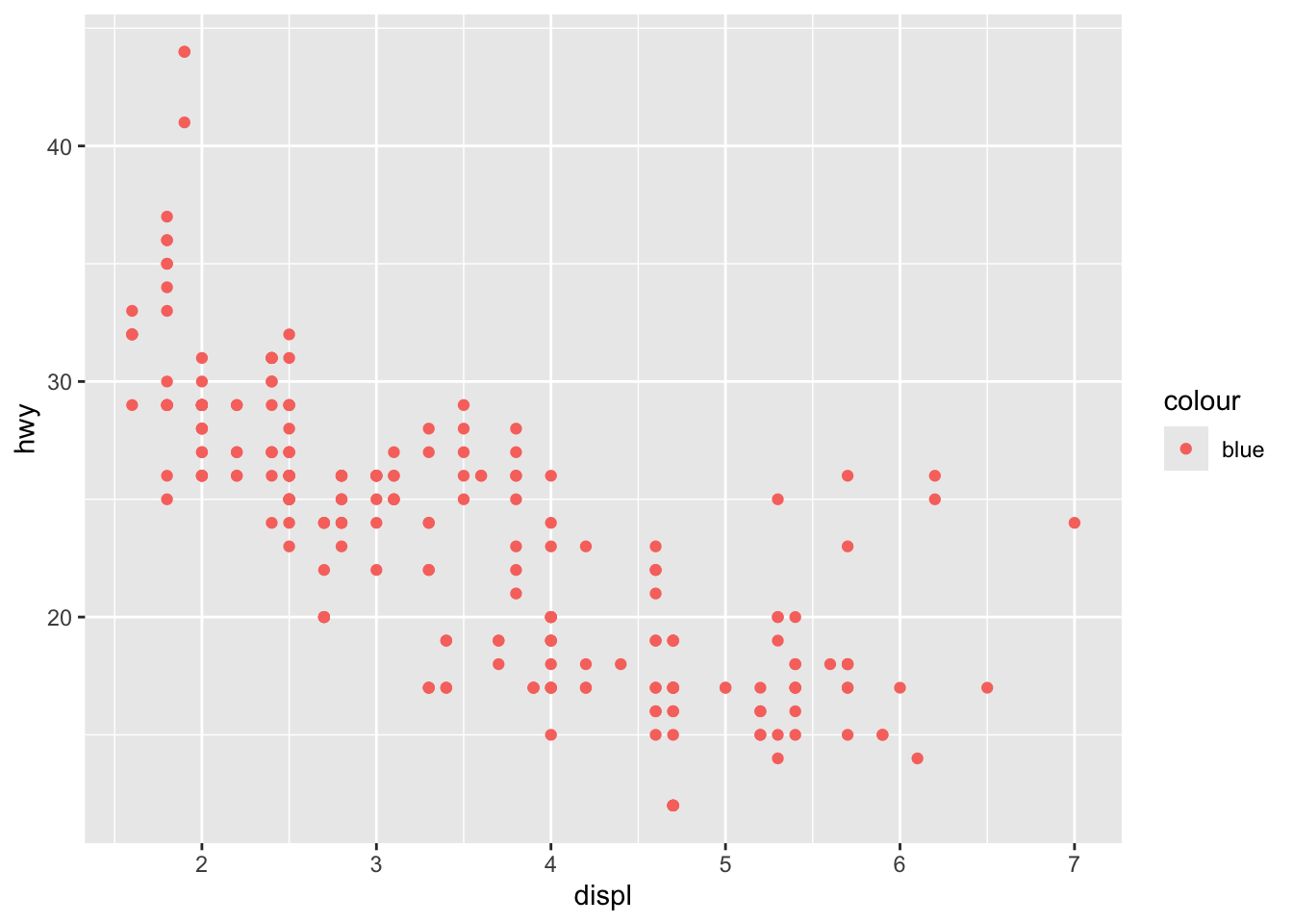
Faceting
ggplot(mpg, aes(displ, hwy)) +
  geom_point() +
  facet_wrap(~ class)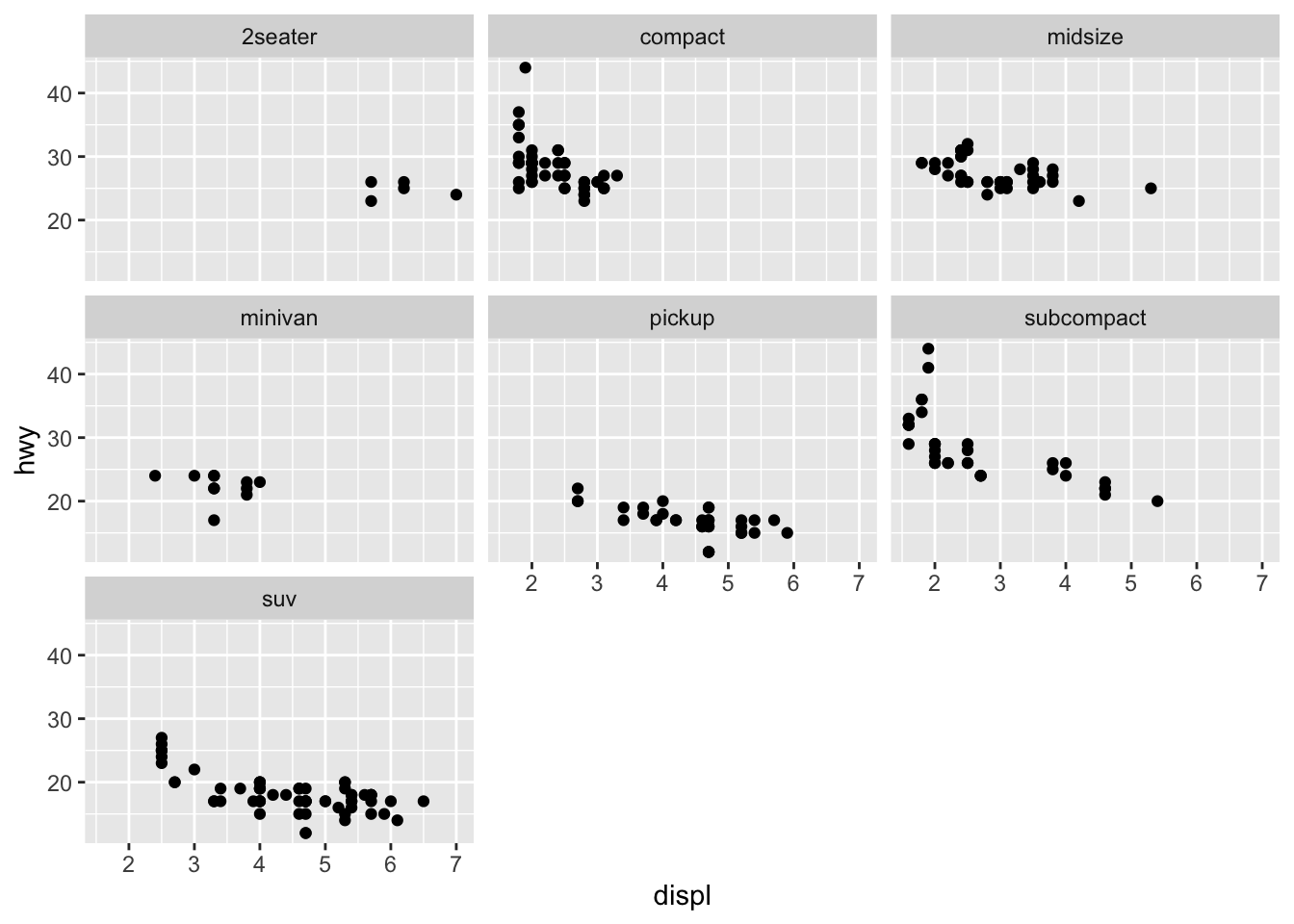
Smoothed trends
ggplot(mpg, aes(displ, hwy)) + geom_point() + geom_smooth()
ggplot(mpg, aes(displ, hwy)) + geom_point() + geom_smooth(method = "lm")
ggplot(mpg, aes(displ, hwy)) + geom_point() + geom_smooth(span = 0.9)  # loess span
`geom_smooth()` using method = 'loess' and formula = 'y ~ x'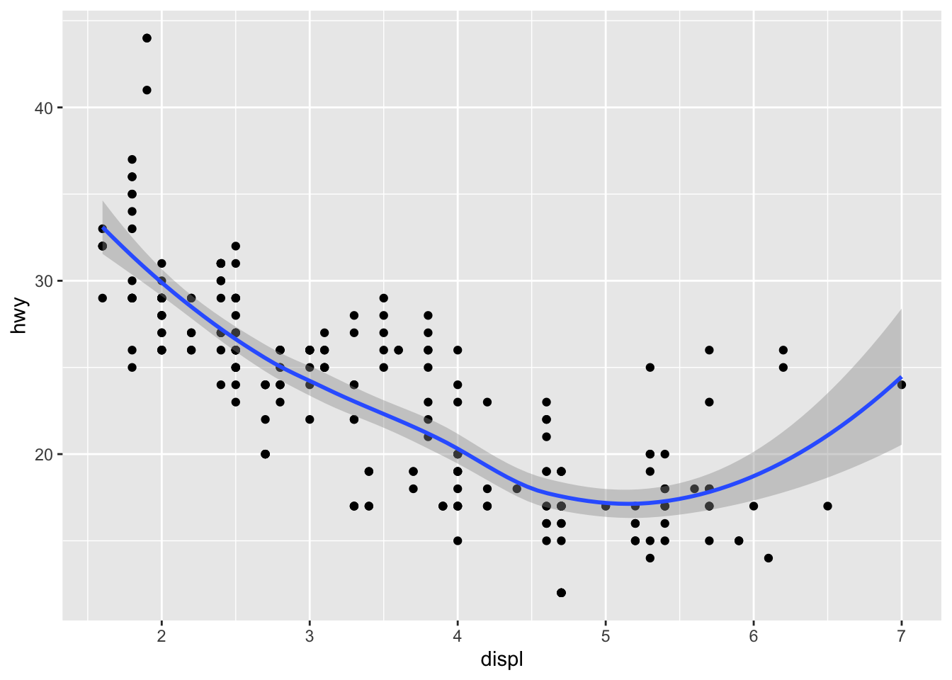
`geom_smooth()` using formula = 'y ~ x'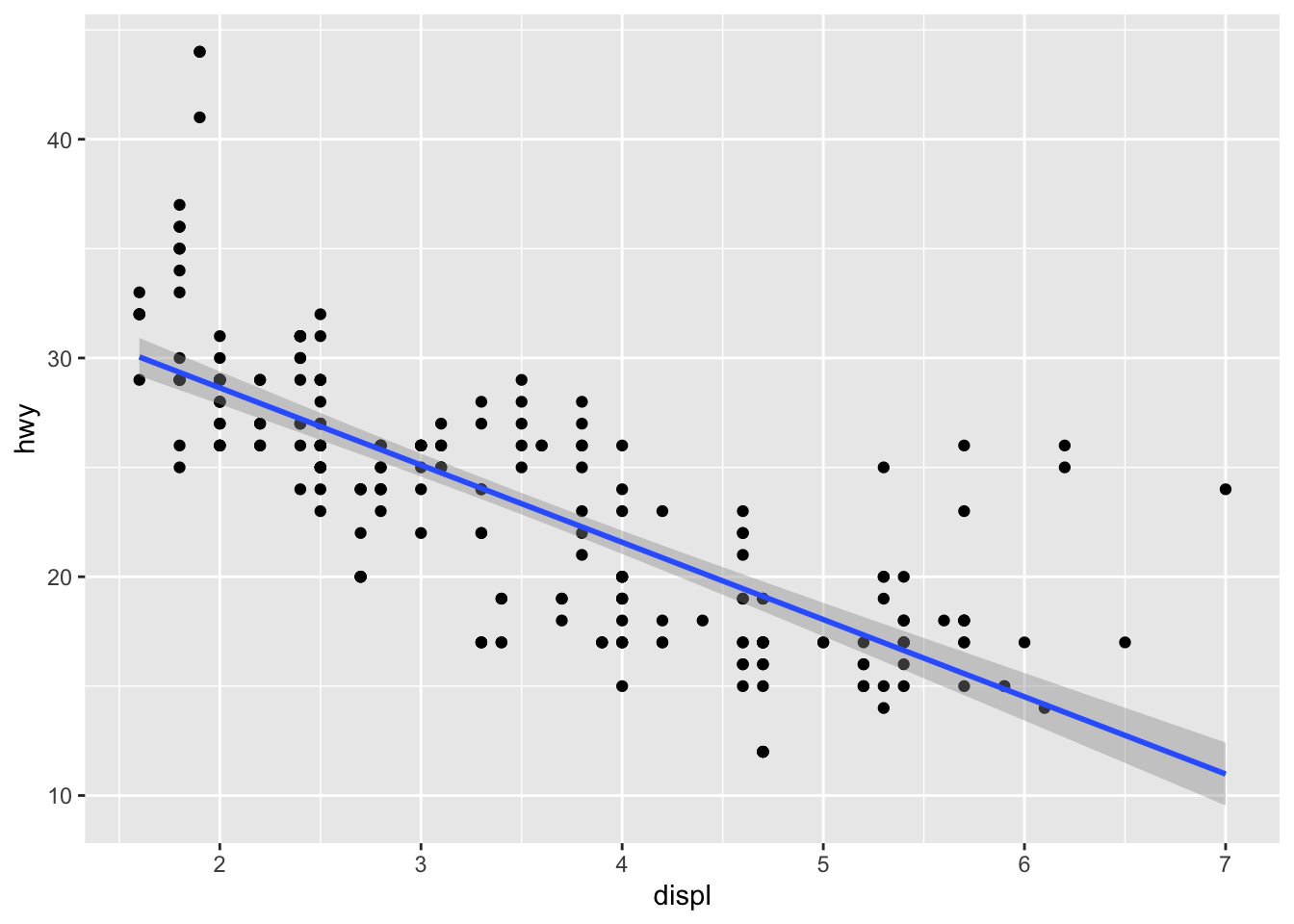
`geom_smooth()` using method = 'loess' and formula = 'y ~ x'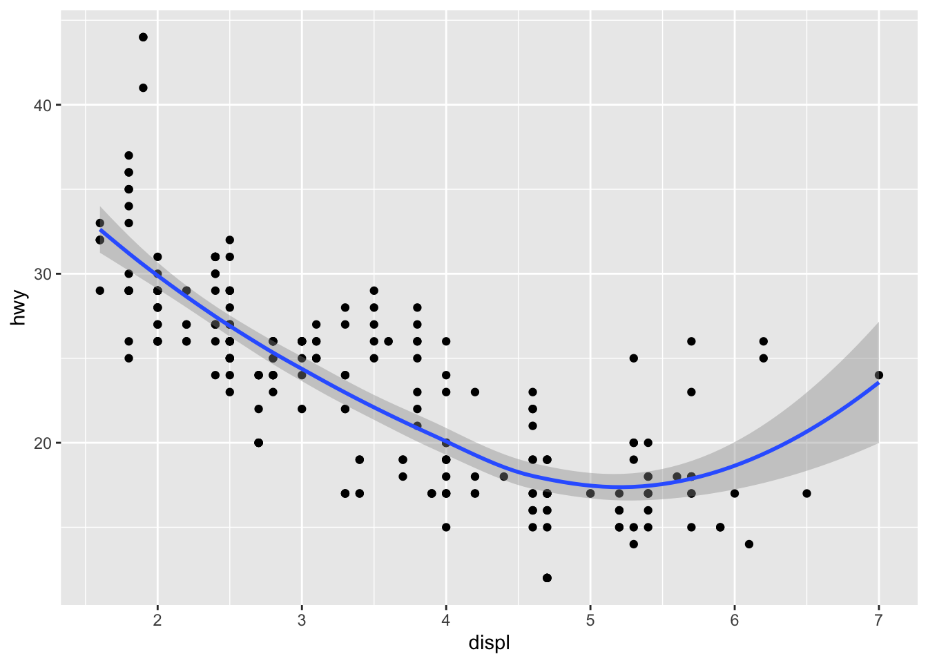
Distributions: histogram, frequency polygon, density, combo
ggplot(mpg, aes(hwy)) + geom_histogram()
ggplot(mpg, aes(hwy)) + geom_freqpoly()
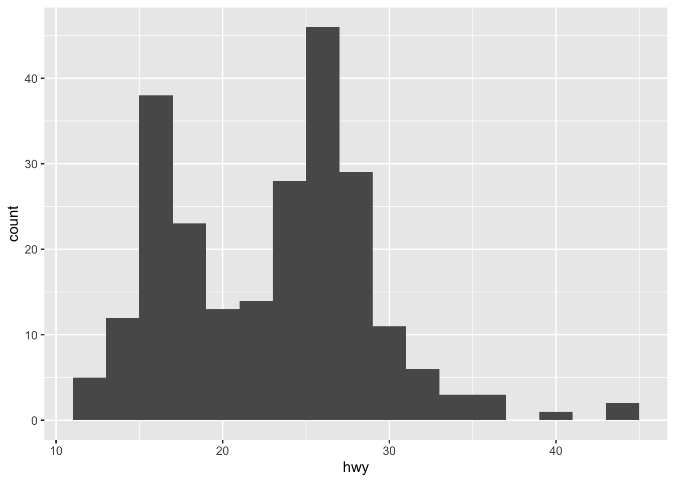
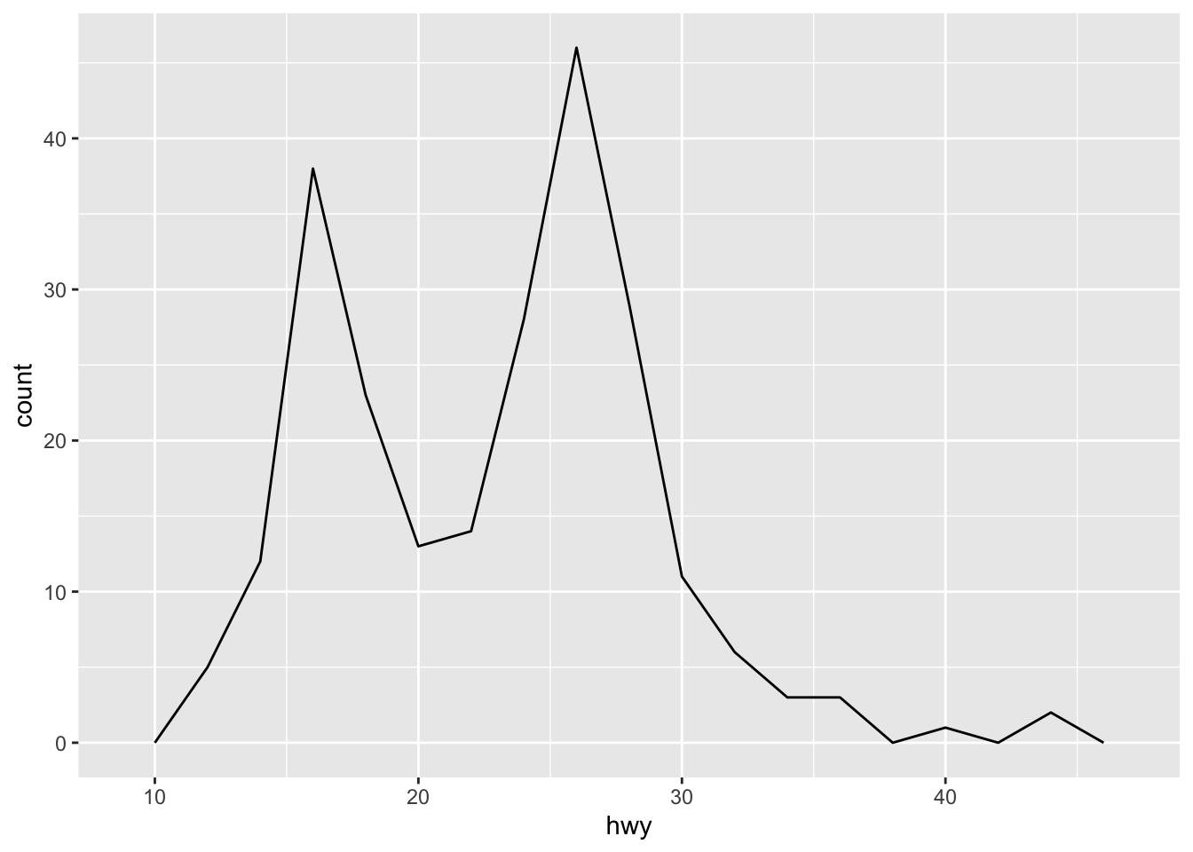
# Change binwidth
ggplot(mpg, aes(hwy)) + geom_histogram(binwidth = 2)
ggplot(mpg, aes(hwy)) + geom_freqpoly(binwidth = 2)
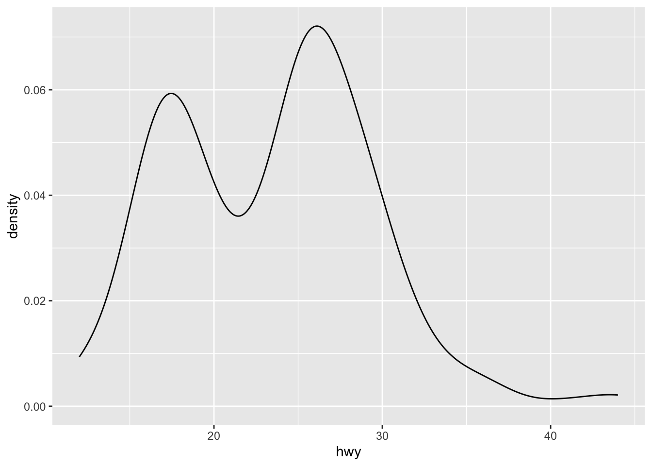
# Density
ggplot(mpg, aes(hwy)) + geom_density()
# Overlay histogram + density and add a mean line
p <- ggplot(mpg, aes(hwy)) +
geom_histogram(aes(y = ..density..), colour = "black", fill = "white") +
geom_density(alpha = .2, fill = "#FF6666")
p + geom_vline(aes(xintercept = mean(hwy)), linetype = "dashed", size = 1)`stat_bin()` using `bins = 30`. Pick better value with `binwidth`.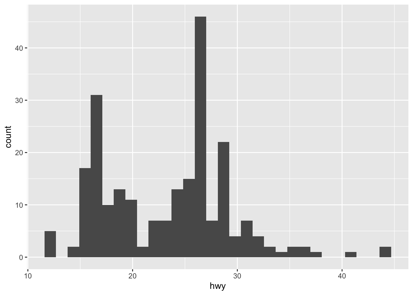
`stat_bin()` using `bins = 30`. Pick better value with `binwidth`.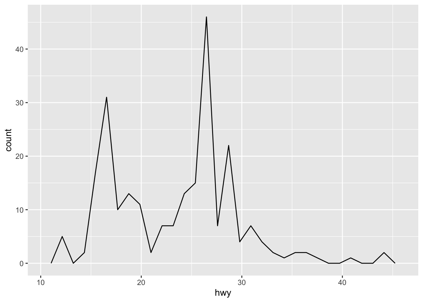
Warning: Using `size` aesthetic for lines was deprecated in ggplot2 3.4.0.
ℹ Please use `linewidth` instead.
Warning: The dot-dot notation (`..density..`) was deprecated in ggplot2 3.4.0.
ℹ Please use `after_stat(density)` instead.`stat_bin()` using `bins = 30`. Pick better value with `binwidth`.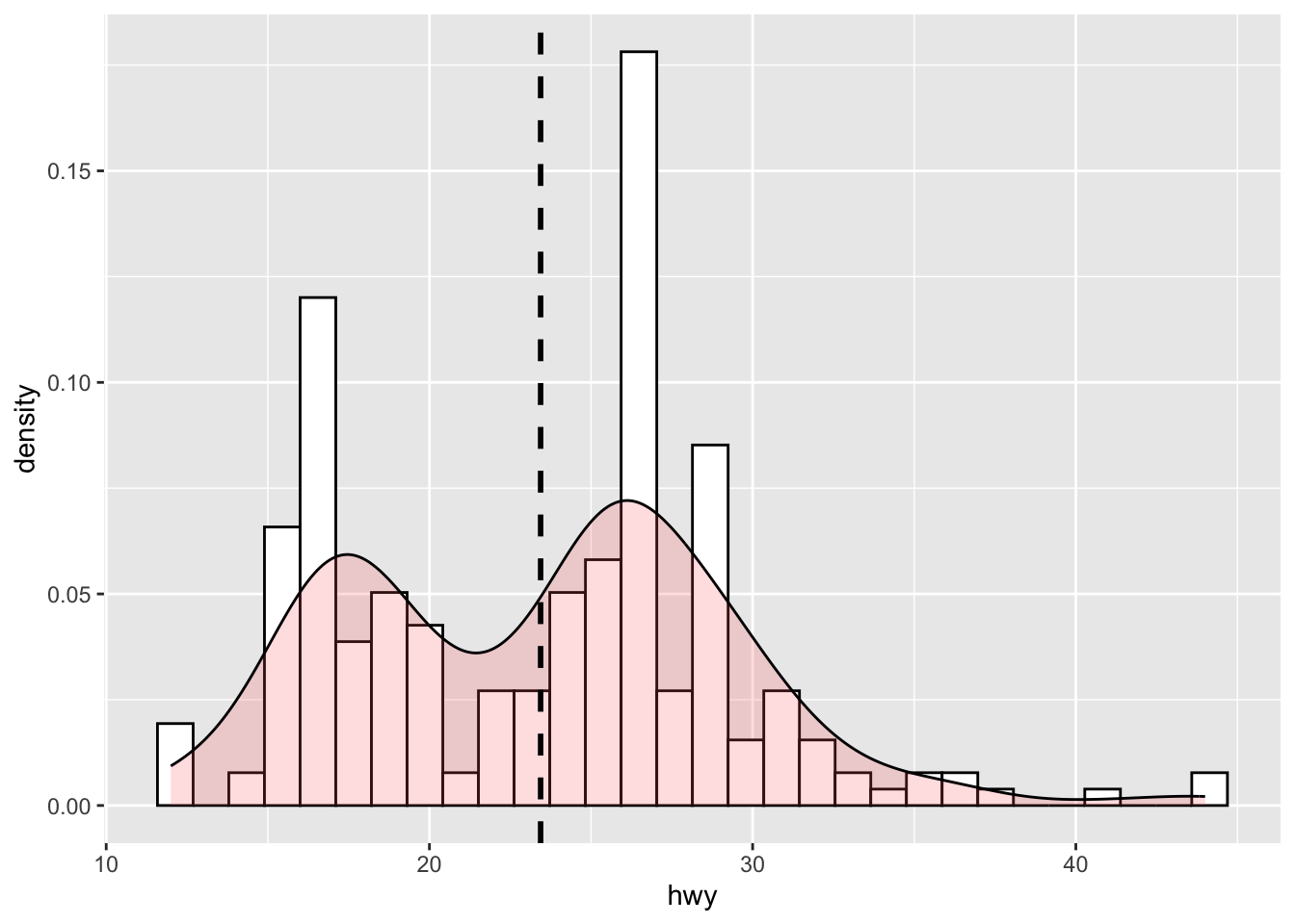
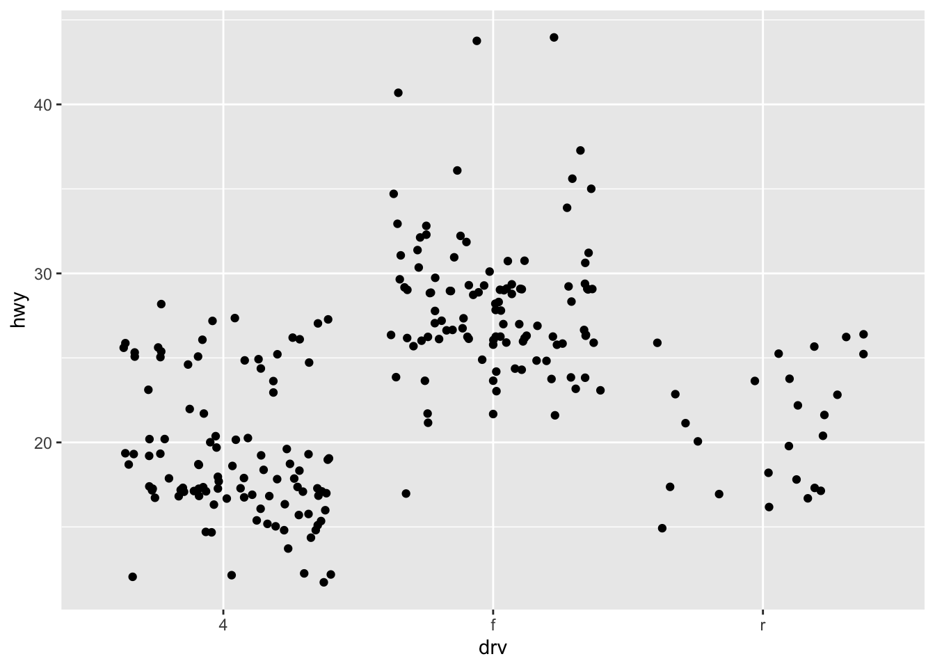
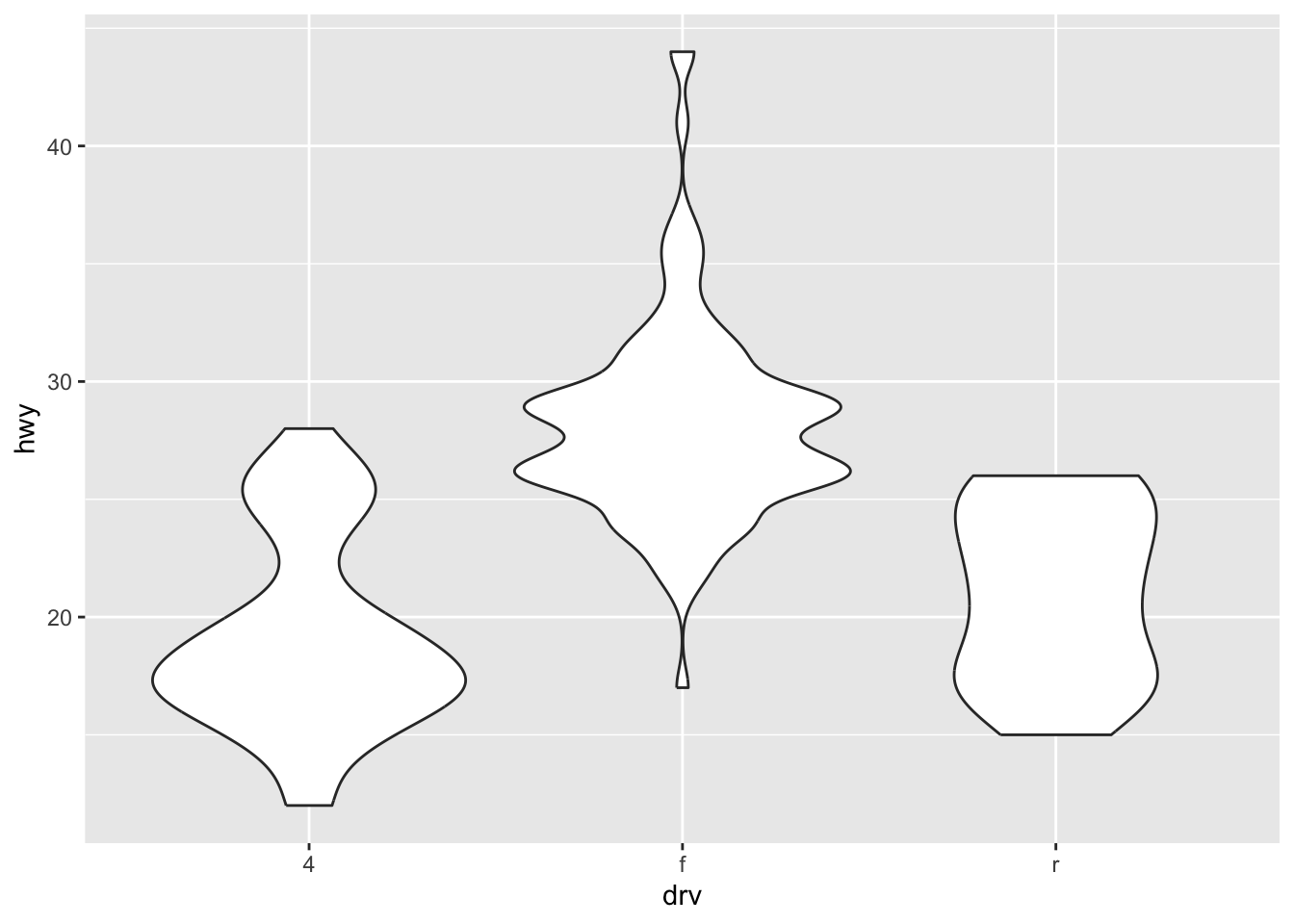
Box, violin, and jitter
ggplot(mpg, aes(drv, hwy)) + geom_boxplot()
ggplot(mpg, aes(drv, hwy)) + geom_jitter()
ggplot(mpg, aes(drv, hwy)) + geom_violin()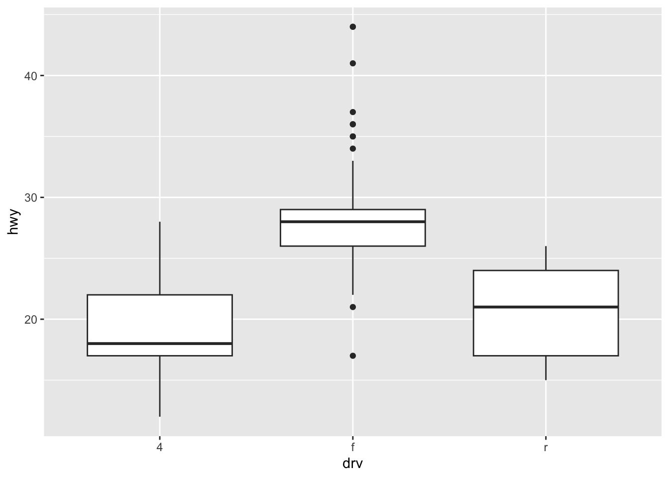
Bars: counts vs. pre-summarised values
# Counts from raw rows
ggplot(mpg, aes(manufacturer)) + geom_bar()
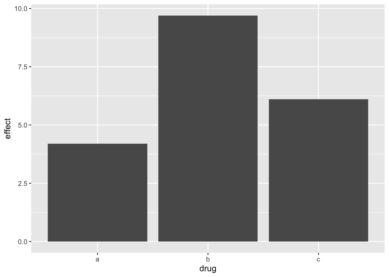
# Pre-summarised data
drugs <- data.frame(
drug = c("a", "b", "c"),
effect = c(4.2, 9.7, 6.1)
)
ggplot(drugs, aes(drug, effect)) + geom_bar(stat = "identity")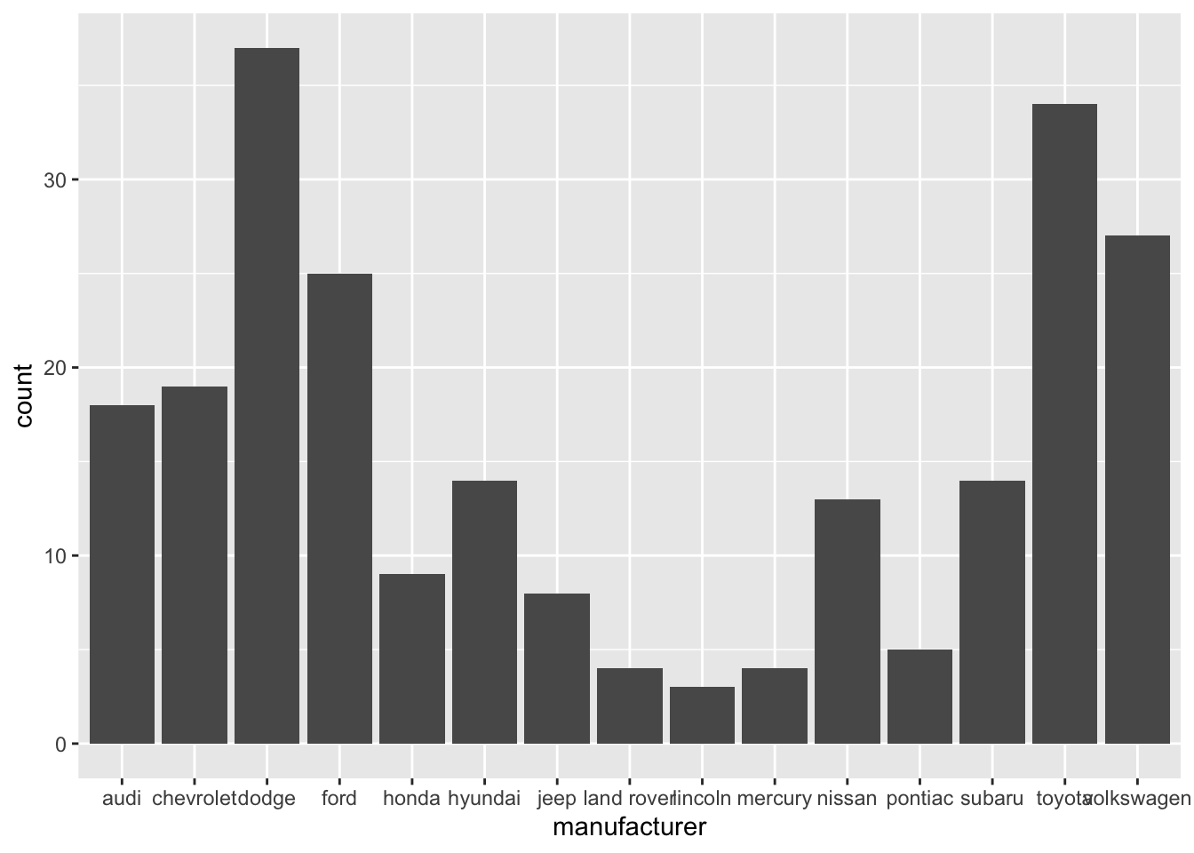
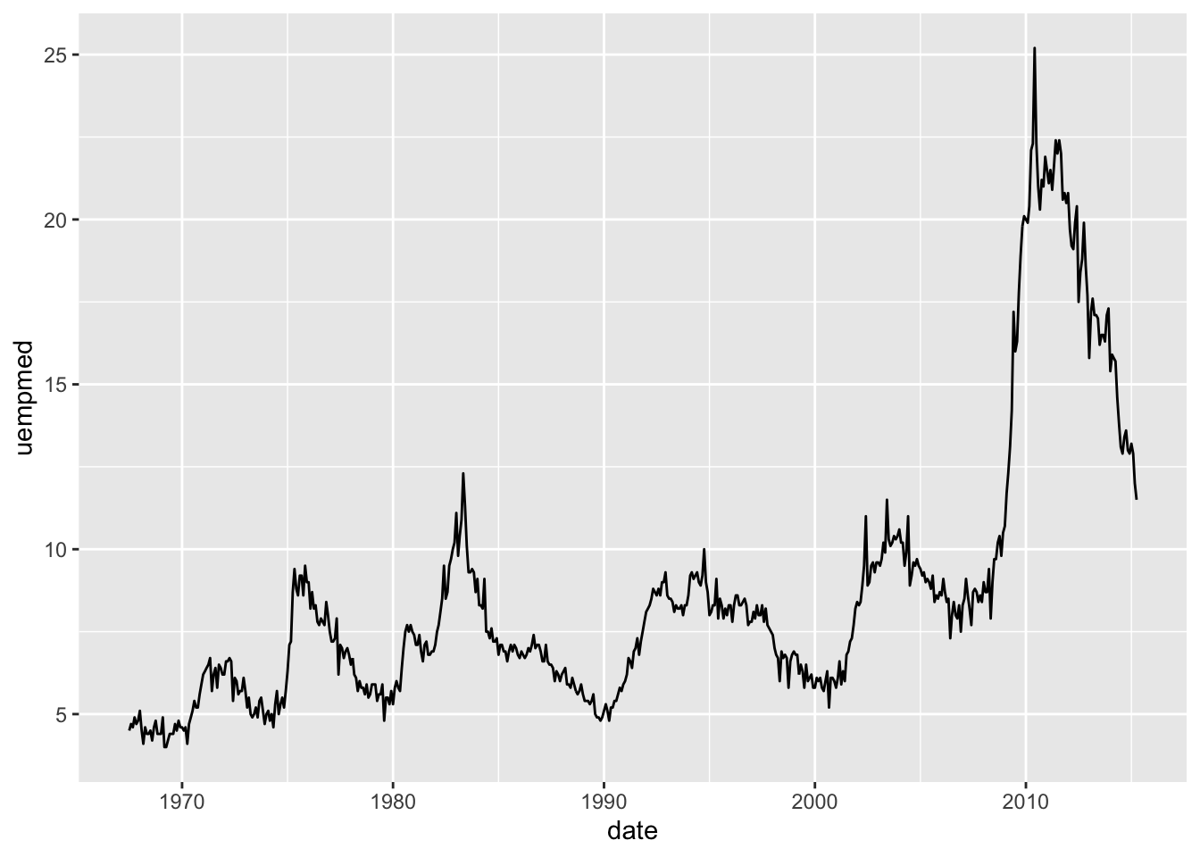
Lines & paths (time series)
ggplot(economics, aes(date, unemploy / pop)) + geom_line()
ggplot(economics, aes(date, uempmed)) + geom_line()

str(economics)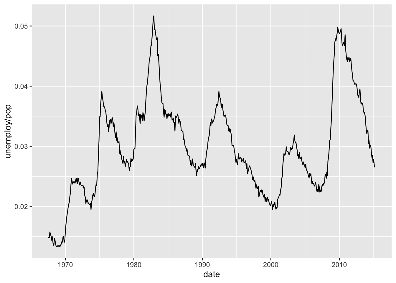
spc_tbl_ [574 × 6] (S3: spec_tbl_df/tbl_df/tbl/data.frame)
 $ date    : Date[1:574], format: "1967-07-01" "1967-08-01" ...
 $ pce     : num [1:574] 507 510 516 512 517 ...
 $ pop     : num [1:574] 198712 198911 199113 199311 199498 ...
 $ psavert : num [1:574] 12.6 12.6 11.9 12.9 12.8 11.8 11.7 12.3 11.7 12.3 ...
 $ uempmed : num [1:574] 4.5 4.7 4.6 4.9 4.7 4.8 5.1 4.5 4.1 4.6 ...
 $ unemploy: num [1:574] 2944 2945 2958 3143 3066 ...
Axes and limits
ggplot(mpg, aes(cty, hwy)) + geom_point(alpha = 1/3)
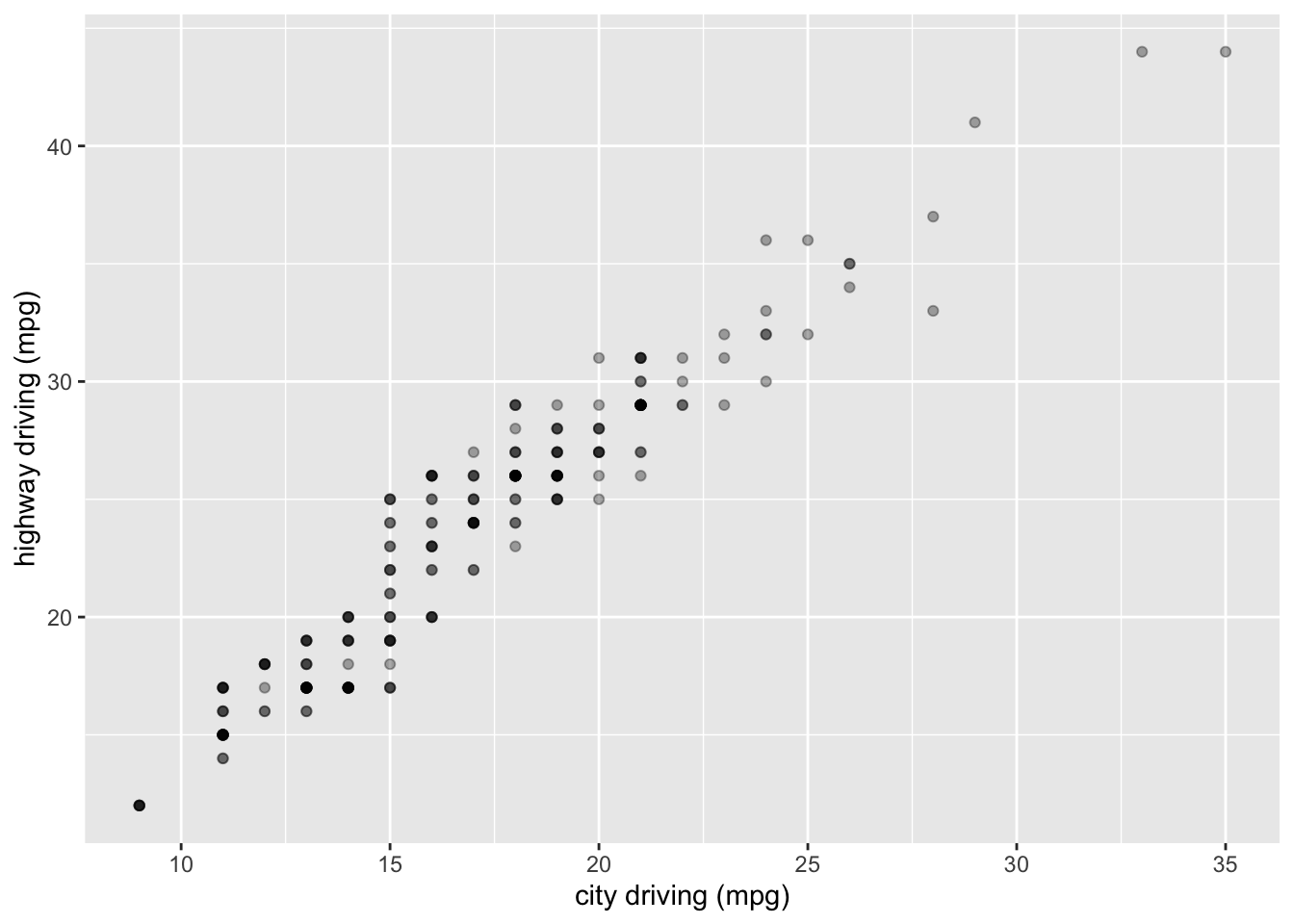
ggplot(mpg, aes(cty, hwy)) +
geom_point(alpha = 1/3) +
xlab("city driving (mpg)") +
ylab("highway driving (mpg)")
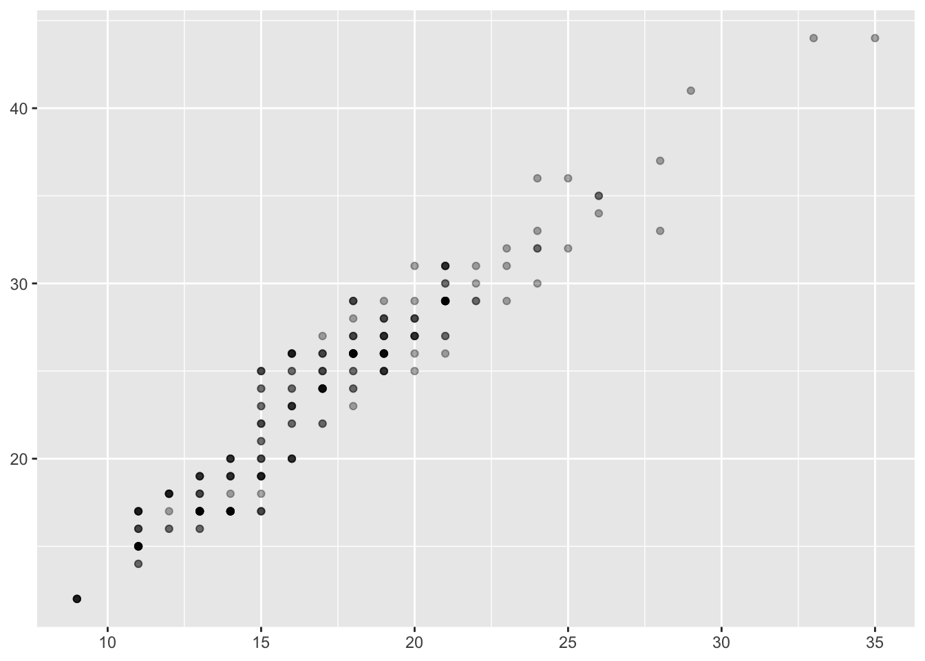
ggplot(mpg, aes(cty, hwy)) + geom_point(alpha = 1/3) + xlab(NULL) + ylab(NULL)
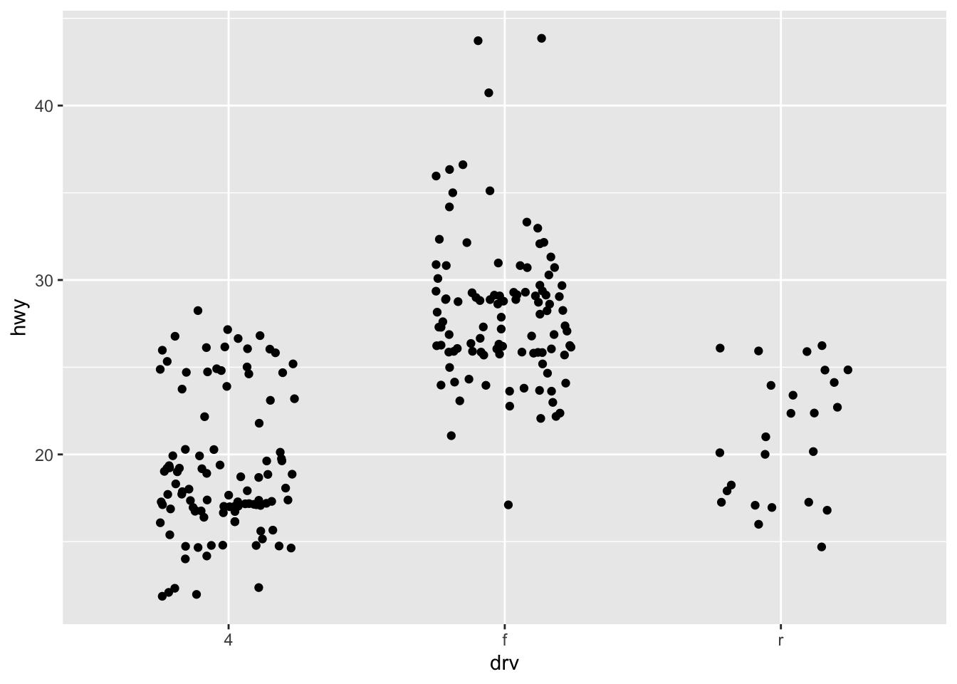
ggplot(mpg, aes(drv, hwy)) + geom_jitter(width = 0.25)
ggplot(mpg, aes(drv, hwy)) +
geom_jitter(width = 0.25) +
xlim("f", "r") +
ylim(20, 30)
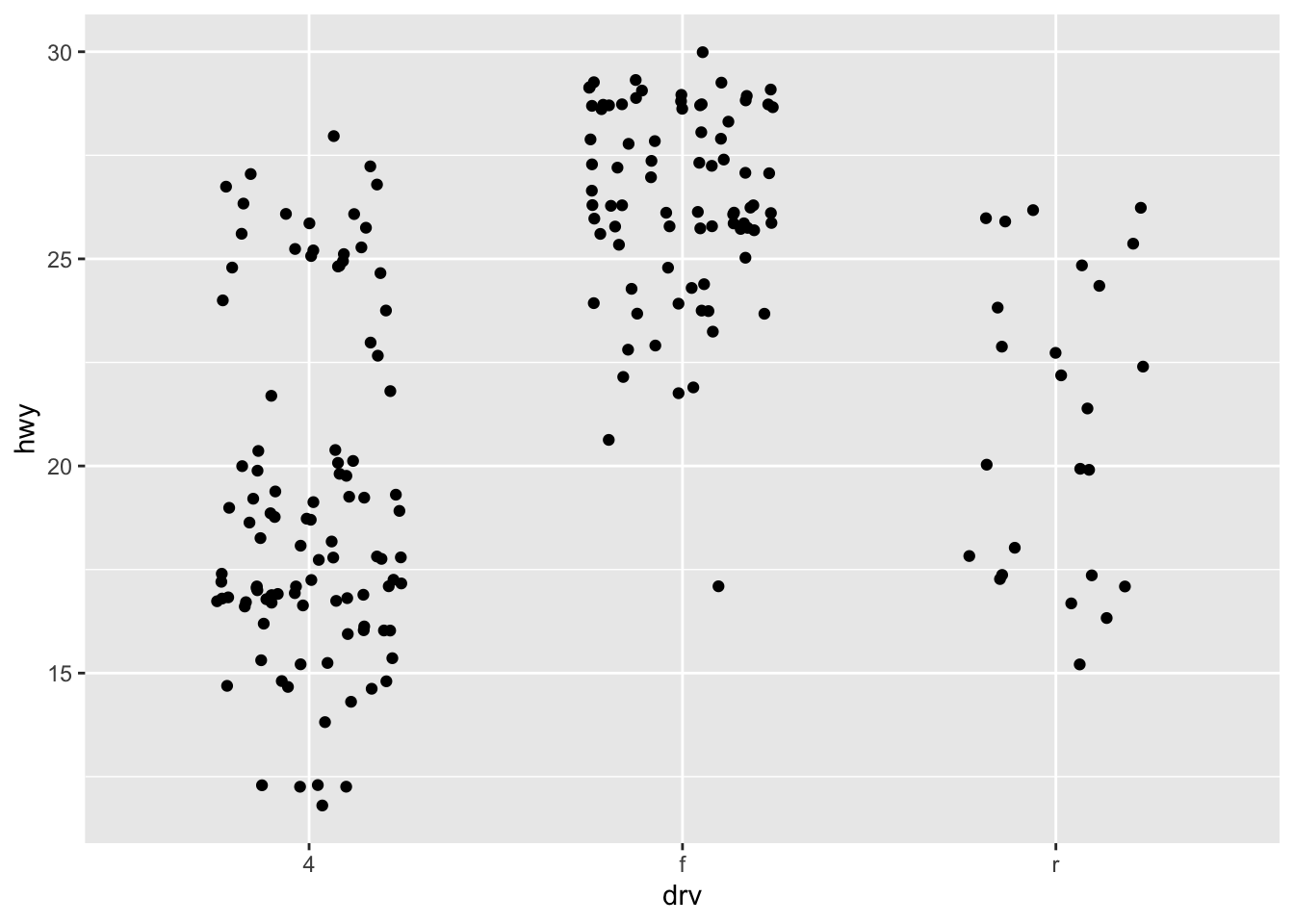
ggplot(mpg, aes(drv, hwy)) +
geom_jitter(width = 0.25, na.rm = TRUE) +
ylim(NA, 30)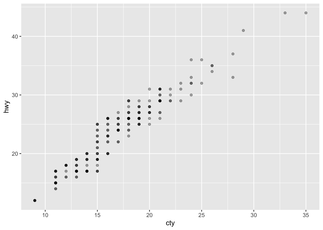
Warning: Removed 139 rows containing missing values or values outside the scale range
(`geom_point()`).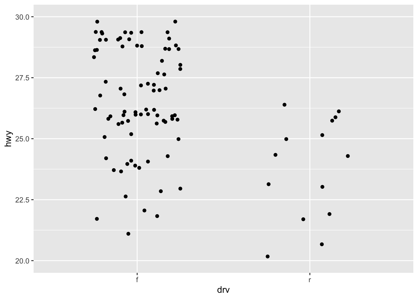
Annotations & math expressions
ggplot(mpg, aes(displ, hwy)) +
geom_point(aes(colour = factor(cyl))) +
labs(
x = "Engine displacement (litres)",
y = "Highway miles per gallon",
colour = "Number of cylinders",
title = "Mileage by engine size and cylinders",
subtitle = "Source: http://fueleconomy.gov"
)
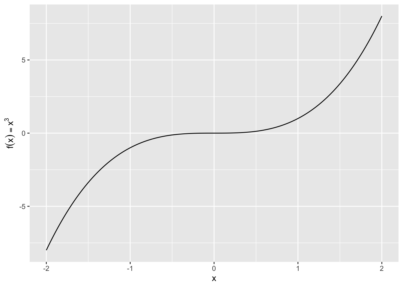
values <- seq(from = -2, to = 2, by = .01)
df <- data.frame(x = values, y = values^3)
ggplot(df, aes(x, y)) +
geom_path() +
labs(y = quote(f(x) == x^3))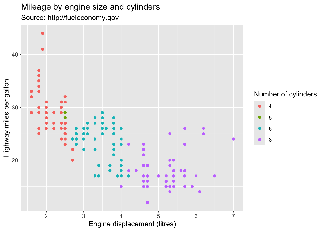
Saving plots
# Save a plot object to disk
p <- ggplot(df, aes(x, y)) +
  geom_path() +
  labs(y = quote(f(x) == x^3))
ggsave("plot.png", p, width = 5, height = 5)

# Or specify a full path you control:
# ggsave("path/to/your/folder/plot.png", p, width = 5, height = 5)
Wrap-up
- Base R conditionals are the building blocks of program logic.
- Base R provides quick descriptive and grouped summaries (
aggregate(),by(),table(),xtabs(),prop.table()). - dplyr enables readable, chained transformations: think rows (
filter()), columns (select(),mutate()), groups (group_by()+summarise()), and joins. - ggplot2 enables layered, expressive visualizations; think in layers and mappings.
Practice: Using mpg, (1) create efficiency with mutate() and case_when(), (2) compute average hwy by class with group_by()/summarise(), and (3) plot hwy vs displ coloured by class with a linear smoother.