Interactions occur when the effect of one independent variable (IV) on the dependent variable (DV) varies depending on the level or value of another IV. This means the relationship between one IV and the DV is contingent upon, or moderated by, another variable.
Conceptually, interactions embody the idea of conditional effects, captured succinctly as relationships that depend on context.
Example: The effect of economic development (GDP per capita) on democratization might depend on the strength of civil society within a country.
Substantively, interactions represent moderation1, where one variable (the moderator) alters the strength, direction, or presence of the relationship between another independent variable and the dependent variable. The moderator is essentially a contextual or contingent factor determining when, how strongly, or even whether a relationship holds.
Example: The impact of trade openness on income inequality could be moderated by the presence or strength of labor unions. Countries with strong labor unions may experience different inequality outcomes compared to those with weak labor unions.
Interpretation
Statistically, interactions are modeled through multiplicative terms in regression equations. Formally, an interaction between variables ( X ) and ( Z ) can be represented as:
The marginal effect of ( X ) depends explicitly on ( Z ): \[
\frac{\partial Y}{\partial X} = \beta_1 + \beta_3Z
\]
Similarly, the marginal effect of ( Z ) depends on ( X ): \[
\frac{\partial Y}{\partial Z} = \beta_2 + \beta_3X
\]
Here, \(\beta_3\) represents the interaction effect, indicating how the relationship between \(X\) and \(Y\) changes with different levels of \(Z\). Or, if \(Z\) is the main IV, then how does \(X\) moderate its relationship to \(Y\)
Key Idea
Interactions formally quantify how relationships change across conditions.
That is, they are used to capture and test conditional hypotheses. Simplest notion of conditional hypothesis is:
\(H_1\): An increase in X is associated with an increase in Y when condition Z is met, but not when condition Z is absent.
Illustrative Example
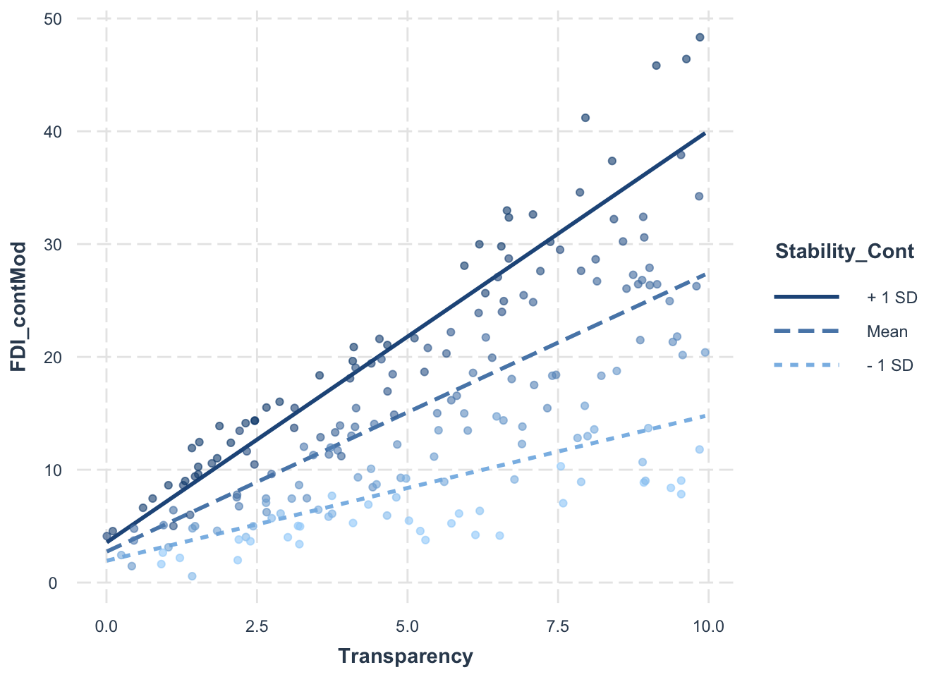
Statistically, if examining how government transparency \(X\) affects foreign direct investment \(Y\), and hypothesizing that this effect depends on political stability \(Z\), the interaction term \(X \times Z\) formally tests and quantifies this conditional relationship.
# Load librarieslibrary(tidyverse)# Set seed for reproducibilityset.seed(123)# Generate dummy datan <-100data <-tibble(Transparency =runif(n, 0, 10),Stability =rep(c(0, 1), each = n/2),epsilon =rnorm(n, 0, 1),FDI =2+0.3*Transparency +1.5*Stability +0.5*Transparency*Stability + epsilon)# Define label positionslabel_data <-tibble(x =c(5.6, 8, 0, 0),y =c(7.5, 4.2, 2, 3.5),label =c("Slope = beta[1] + beta[3]", "Slope = beta[1]", "beta[0]", "+beta[2]"),Stability =factor(c(1, 0, 0, 1)))# Plot the interaction using ggplot(p1 <-ggplot(data, aes(x = Transparency, y = FDI, color =factor(Stability))) +geom_point(alpha =0.3) +geom_smooth(method ="lm", se =FALSE, formula = y ~ x) +geom_text(data = label_data, aes(x = x, y = y, label = label), parse =TRUE, color ="black", size =5, hjust =0) +scale_color_manual(values =c("blue", "red"), labels =c("Stability = Low", "Stability = High")) +labs(title ="Effect of Transparency on FDI Conditional on Stability",x ="Government Transparency",y ="Foreign Direct Investment (FDI)",color ="Political Stability" ) +annotate("text", x =3, y =10, label ="FDI == (beta[0]+beta[2])+(beta[1]+beta[3])*Transparency~when~Stability==1", parse =TRUE, hjust =0, size =3.5) +annotate("text", x =3, y =2.5, label ="FDI == beta[0]+beta[1]*Transparency~when~Stability==0", parse =TRUE, hjust =0, size =3.5) +theme_minimal() +theme(legend.position ="bottom" ))
The data and relationship displayed in the plot above was generated using the following equation \[
\text{FDI} = 2 + 0.3\,(\text{Transparency}) + 1.5\,(\text{Stability}) + 0.5\,(\text{Transparency} \times \text{Stability}) + \epsilon
\]
# Linear regression model with binary moderatormodel_binary <-lm(FDI_binaryMod ~ Transparency * Stability_Binary, data = data)summary(model_binary)
Call:
lm(formula = FDI_binaryMod ~ Transparency * Stability_Binary,
    data = data)

Residuals:
     Min       1Q   Median       3Q      Max
-2.82901 -0.66817  0.04696  0.68887  2.44328

Coefficients:
                              Estimate Std. Error t value Pr(>|t|)
(Intercept)                    2.21076    0.20156  10.968  < 2e-16 ***
Transparency                   0.35538    0.03427  10.369  < 2e-16 ***
Stability_Binary               1.21044    0.30522   3.966 0.000103 ***
Transparency:Stability_Binary  0.61978    0.05337  11.613  < 2e-16 ***
---
Signif. codes:  0 '***' 0.001 '**' 0.01 '*' 0.05 '.' 0.1 ' ' 1

Residual standard error: 1.015 on 196 degrees of freedom
Multiple R-squared:  0.8869,    Adjusted R-squared:  0.8852
F-statistic: 512.5 on 3 and 196 DF,  p-value: < 2.2e-16
// Linear regression model with binary moderatorreg FDI_binaryMod c.Transparency##i.Stability_Binary
Interpretation: The interaction term shows how the relationship between Transparency and FDI differs across Stability_Binary groups (0 vs. 1).
Statistically, the interaction term Transparency:Stability_Binary has a coefficient of 0.61978 and is highly statistically significant (p < 0.001). This indicates strong statistical evidence that the effect of Transparency on FDI increases significantly as Stability_Cont increases.
Substantively, the positive interaction term suggests that higher political stability (Stability_Cont) enhances the beneficial impact of government transparency (Transparency) on attracting foreign direct investment (FDI). In other words, transparency leads to even greater increases in FDI when combined with a stable political environment.
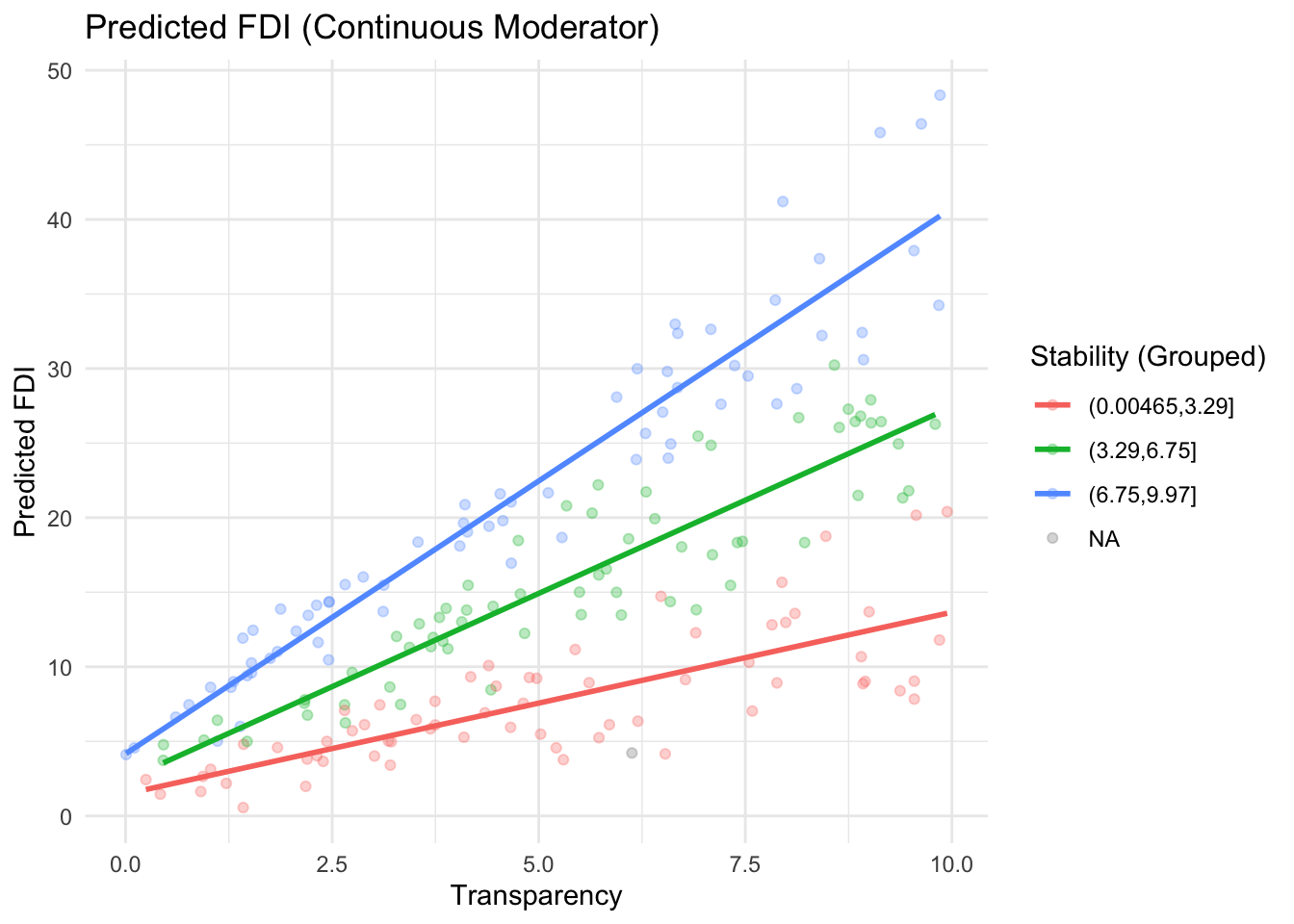
Predicted Outcome Plot (Binary Moderator)
We visualize how predicted FDI varies across Transparency levels for each group defined by the binary moderator.
Recall, the marginal effect of \(X\) depends explicitly on \(Z\): \[
\frac{\partial Y}{\partial X} = \beta_1 + \beta_3Z
\] The coefficient of our main variable of interest \(X\) changes at different values of Z. Let’s vizualize that.
The interplot package allows visualization of how the marginal effect of one variable on the outcome changes across the values of another (moderator) variable.
First, ensure you’ve installed the package:
#install.packages("interplot")library(interplot)# Plot marginal effect of Transparency on FDI for each Stability_Binary categoryinterplot(m = model_binary, var1 ="Transparency", var2 ="Stability_Binary") +labs(x ="Stability (Binary)", y ="Marginal Effect of Transparency", title ="Marginal Effect of Transparency by Stability (Binary)") +theme_minimal()
// Marginal effect plotmargins Stability_Binary, dydx(Transparency)marginsplot, ///xlabel(0 1, valuelabel) ///title("Marginal Effect of Transparency by Stability (Binary)") ///xtitle("Stability (Binary)") ///ytitle("Marginal Effect of Transparency")
Interpretation: This plot displays the marginal effect of Transparency on FDI for the two groups defined by the binary Stability moderator. Points represent the marginal effects, with lines indicating the 95% confidence intervals.
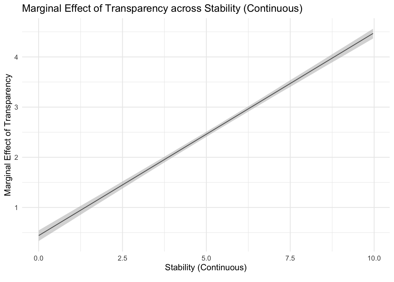
library(interplot)# Plot marginal effect of Transparency on FDI across Stability_Continterplot(m = model_cont, var1 ="Transparency", var2 ="Stability_Cont") +labs(x ="Stability (Continuous)", y ="Marginal Effect of Transparency", title ="Marginal Effect of Transparency across Stability (Continuous)") +theme_minimal()
// Marginal effect plotmargins, dydx(Transparency) at(Stability_Cont=(0(1)10))marginsplot, ///xlabel(0(1)10) ///title("Marginal Effect of Transparency across Stability (Continuous)") ///xtitle("Stability (Continuous)") ///ytitle("Marginal Effect of Transparency")
Interpretation: This plot shows how the marginal effect (coefficient) of Transparency on FDI changes at different values of Stability (Continuous). The shaded area (in R) or error bars (in Stata) indicates the 95% confidence interval.
Guiderails
In a paper highly cited for formalizing the practice around usage and reporting of multiplicative-interaction models, Brambor, Clark, and Golder (2006) list three instructions which have become a norm in analysis since then:
Include in the model all constitutive terms (Z and X) alongside the interaction term (Z \(\times\) X).
Not interpret the coefficients on the constitutive terms as unconditional marginal effects.
Compute substantively meaningful marginal effects and confidence intervals, ideally with a plot that shows how the conditional marginal effect of X on Y changes across levels of the moderator Z.
Applying these guidelines to our examples:
First, our models correctly include both constitutive terms (Transparency and Stability) alongside the interaction term, thus avoiding omitted-variable bias and ensuring accurate estimation of conditional effects.
Second, we interpret coefficients appropriately, recognizing that the main coefficients for Transparency or Stability alone cannot be interpreted independently because their meaning is conditioned on the other variable. We focus explicitly on the interaction terms to understand conditional relationships.
Third, we demonstrate and visualize substantively meaningful conditional effects by plotting predicted values across different levels of our moderators (both binary and continuous), clearly illustrating how the relationship between Transparency and FDI varies conditionally.
Advanced Issues
More recently, methodology scholarship has highlighted some finer issues with the analysis and reporting of results from multiplicative interaction models. In case your project uses interactions and you want to make it publication ready in the future, you may consult discussion of advanced issues here
Additional Resources
Kam, C. D., & Franzese, R. J. (2007). Modeling and Interpreting Interactive Hypotheses in Regression Analysis. University of Michigan press.
Brambor, T., Clark, W. R., & Golder, M. (2006). Understanding Interaction Models: Improving Empirical Analyses. Political Analysis, 14(1), 63–82. https://www.jstor.org/stable/25791835.2
Esarey, J., & Sumner, J. L. (2018). Marginal Effects in Interaction Models: Determining and Controlling the False Positive Rate. Comparative Political Studies, 51(9), 1144–1176. https://doi.org/10.1177/00104140177300803
Hainmueller, J., Mummolo, J., & Xu, Y. (2019). How Much Should We Trust Estimates from Multiplicative Interaction Models? Simple Tools to Improve Empirical Practice. Political Analysis, 27(2), 163–192. https://doi.org/10.1017/pan.2018.464
Brambor, Thomas, William Roberts Clark, and Matt Golder. 2006. “Understanding Interaction Models: Improving Empirical Analyses.”Political Analysis 14 (1): 63–82. https://www.jstor.org/stable/25791835.
Moderation is a widely-used interpretation.However, interactions are a versatile analytical tool capable of capturing diverse relationships between variables, including complementarity, substitution, context-dependency, nonlinearity, and effect heterogeneity↩︎
Abstract:Multiplicative interaction models are common in the quantitative political science literature. This is so for good reason. Institutional arguments frequently imply that the relationship between political inputs and outcomes varies depending on the institutional context. Models of strategic interaction typically produce conditional hypotheses as well. Although conditional hypotheses are ubiquitous in political science and multiplicative interaction models have been found to capture their intuition quite well, a survey of the top three political science journals from 1998 to 2002 suggests that the execution of these models is often flawed and inferential errors are common. We believe that considerable progress in our understanding of the political world can occur if scholars follow the simple checklist of dos and don’ts for using multiplicative interaction models presented in this article. Only 10% of the articles in our survey followed the checklist.↩︎
Abstract:When a researcher suspects that the marginal effect of x on y varies with z, a common approach is to plot ∂y/∂x at different values of z along with a pointwise confidence interval generated using the procedure described in Brambor, Clark, and Golder to assess the magnitude and statistical significance of the relationship. Our article makes three contributions. First, we demonstrate that the Brambor, Clark, and Golder approach produces statistically significant findings when ∂y/∂x=0 at a rate that can be many times larger or smaller than the nominal false positive rate of the test. Second, we introduce the interactionTest software package for R to implement procedures that allow easy control of the false positive rate. Finally, we illustrate our findings by replicating an empirical analysis of the relationship between ethnic heterogeneity and the number of political parties from Comparative Political Studies.↩︎
Abstract:Multiplicative interaction models are widely used in social science to examine whether the relationship between an outcome and an independent variable changes with a moderating variable. Current empirical practice tends to overlook two important problems. First, these models assume a linear interaction effect that changes at a constant rate with the moderator. Second, estimates of the conditional effects of the independent variable can be misleading if there is a lack of common support of the moderator. Replicating 46 interaction effects from 22 recent publications in five top political science journals, we find that these core assumptions often fail in practice, suggesting that a large portion of findings across all political science subfields based on interaction models are fragile and model dependent. We propose a checklist of simple diagnostics to assess the validity of these assumptions and offer flexible estimation strategies that allow for nonlinear interaction effects and safeguard against excessive extrapolation. These statistical routines are available in both R and STATA.↩︎