Session 5 - Moderation

“… It’s something unpredictable
But in the end, it’s right
I hope you had the time of your life”,

- Greenday, realising the potential of non-parametric estimation from data in finding non-linearities, through the song Good Riddance

Material

1. Download the 8003-Moderation Lab folder from here.

2. Run the .RProj file.

3. Open 8003-moderation-11262024.qmd.

Today’s Lab

1. Heterogeneous Effects of Same Treatment

2. How to analyse moderation?

3. Moderation using interflex package

4. In-class Exercise

Heterogeneous Effects of Same Treatment

We have studied a a range of concepts (in this class and before) that look at how an expnlanatory variable (or \(treatment\)) can have its relationship with dependent variable (or \(outcome\)) vary according other another variable (moderator or mediator). A year and a half ago, it was covered as \(interactions\) in Govt 8001, as \(moderator\) in Govt 8002, and in Govt 8003 we have talked about \(treatment-effect-heterogeneity\). Additionally, we have also talked about \(mediation\) which conceptually has a similar skeleton, with the major change being that of context i.e identifying whether and how the above relationship varies through a particular path (causal mechanisms, that it).

Arguably, they have similarities in mechanics, both mathematically and statistically. The table below looks at how and when all these terms are used.

Concepts and Usage

Concept	Question It Answers	Example
Treatment Effect Heterogeneity	Does the treatment effect vary across groups?	A get-out-the-vote campaign is more effective in swing districts than in safe districts.
Interaction	Does (X)’s effect on (Y) depend on (Z)?	The effect of campaign spending ((X)) on voter turnout ((Y)) depends on voter education levels (\(Z\))).
Moderation	When or for whom does (X \(\to\) Y)?	The relationship between political advertisements ((X)) and voter persuasion ((Y)) is stronger for undecided voters ((Z)).
Mediation	How or why does (X \(\to\) Y)?	Economic inequality ((X)) increases political polarization ((Y)) by reducing trust in institutions ((M)).

Below, we see how despite having same mechanistic underpinnings, these terms have different usage and critically - different aims in knowledge production.

Key Differences and Overlap

Aspect	Treatment Effect Heterogeneity	Interaction	Moderation	Mediation
Focus	Studies variability in treatment effects across groups.	Examines joint effects: Does (X)’s effect on (Y) depend on another variable?	Examines when, where, or for whom (X \(\to\) Y) occurs.	Explains how or why (X \(\to\) Y) happens.
Key Question	Does the effect of (X) vary across subgroups?	Do (X) and another variable combine to influence (Y)?	Does a third variable influence the strength/direction of (X \(\to\) Y)?	What is the pathway from (X) to (Y)?
Causal or Statistical	Causal (subgroup differences).	Statistical (interaction terms).	Statistical (often causally interpreted).	Causal (pathways/mechanisms).
Methodology	Interaction terms, subgroup analysis.	Interaction terms in regression.	Interaction terms in regression.	Path analysis, structural equation modeling.
Example	Get-out-the-vote campaigns are more effective in swing districts than safe ones.	Campaign spending ((X)) affects voter turnout ((Y)) differently based on education ((Z)).	Social media use ((X)) affects political knowledge ((Y)) more for younger voters ((Z)).	Economic inequality ((X)) increases polarization ((Y)) via reduced institutional trust ((M)).
Overlap	Can be explained by mediation (pathways) or tested via interactions.	Often used to model both treatment heterogeneity and moderation.	Moderation can influence mediation pathways (moderated mediation).	Mechanisms can interact with moderators or vary across groups.

Treatment Effect Heterogeneity can arise due to both mediation and moderation.

Moderation occurs when the relationship between a treatment (or independent variable X) and an outcome (or dependent variable Y) changes depending on a third variable (the moderator Z). Moderation explains heterogeneity when the effect of the treatment on the outcome differs for different levels or categories of the moderator variable.

Mediation involves understanding how or why a treatment has an effect on the outcome through an intervening variable (the mediator M). Treatment effect heterogeneity can arise if the mediating pathway varies across different subgroups or conditions. Mediation explains heterogeneity when the process or pathway through which the treatment influences the outcome differs between subgroups.

Example

Suppose we are studying a voter turnout campaign (treatment X) and its impact on voter turnout (outcome Y).

• Moderation Example: The effect of the campaign on voter turnout might be stronger for young voters than for older voters. Age (Z) moderates the effect of the treatment on the outcome.

• Mediation Example: The campaign increases trust in the political system (mediator M), and trust is what drives higher voter turnout. However, the mediating effect of trust might be stronger for younger voters than for older voters, creating heterogeneity in the treatment effect due to the mediation pathway.

Lastly, interaction is the statistical concept that underpins the investigation of either of these.

How to analyse Moderation?

Well, by including interaction term/s in our model.

\[ Y = \beta_0 + \beta_1 D + \beta_2 X + \beta_3 D \times X + \gamma \mathbf{Z} + \epsilon \]

where, D is our binary treatment and X is a moderator (could be continuous or discrete), and \(\mathbf{Z}\) are other control variables.

This model allows for testing of conditional hypothesis of the form:

\(H_1\): The increase in \(Y\) is associated with change in D when condition X is present, but not when X is absent.

In a paper highly cited for formalizing the practice around usage and reporting of multiplicative-interaction models of the above form, Brambor, Clark, and Golder (2006), list out three instructions which have become a norm in analysis since then (Hainmueller, Mummolo, and Xu 2019). These are:

1. Include in the model all constitutive terms (D and X ) alongside the interaction term (D \(\times\) X ).
   
2. Not interpret the coefficients on the constitutive terms (\(\beta_1\) and \(\beta_2\)) as unconditional marginal effects.
   
3. Compute substantively meaningful marginal effects and confidence intervals, ideally with a plot that shows how the conditional marginal effect of D on Y changes across levels of the moderator X.

Hainmueller, Mummolo, and Xu (2019) contend that despite these norms, the practice and reporting of multiplicative-interaction has flaws. They distill them into two overlooked assumptions that the estimation of such models depend on:

1. Linear Interaction Assumption (LIE): The assumption that the effect of the treatment variable on the outcome variable changes linearly with the moderator variable. That is, interaction effect is linear and follows the functional form:

\[\frac{\partial Y}{\partial D} = \beta_1 + \beta_3 X\] The LIE assumption suggests that the heterogeneity in effects is such that for every one-unit increase in X, the effect of D on Y changes by \(\beta_3\), and this change in the effect remains constant across the entire range of X.

2. Common support: The range of values for the moderator variable where there are observations for both the treatment and control groups. To compute the marginal effect of \(D\) at a given value of the moderator, \(x_0\)​, two conditions must ideally be met:
   

1. there should be enough observations with X values close to \(x_0\), and
   
2. there must be variation in the treatment D at \(x_0\).

If either condition is not met, the estimates of the conditional marginal effect rely on extrapolation or interpolation of the functional form into regions with little or no data. As a result, these effect estimates become fragile and highly dependent on the model used (King and Zeng 2006).

Solution

Hainmueller, Mummolo, and Xu (2019) propose few remedies to the issues.

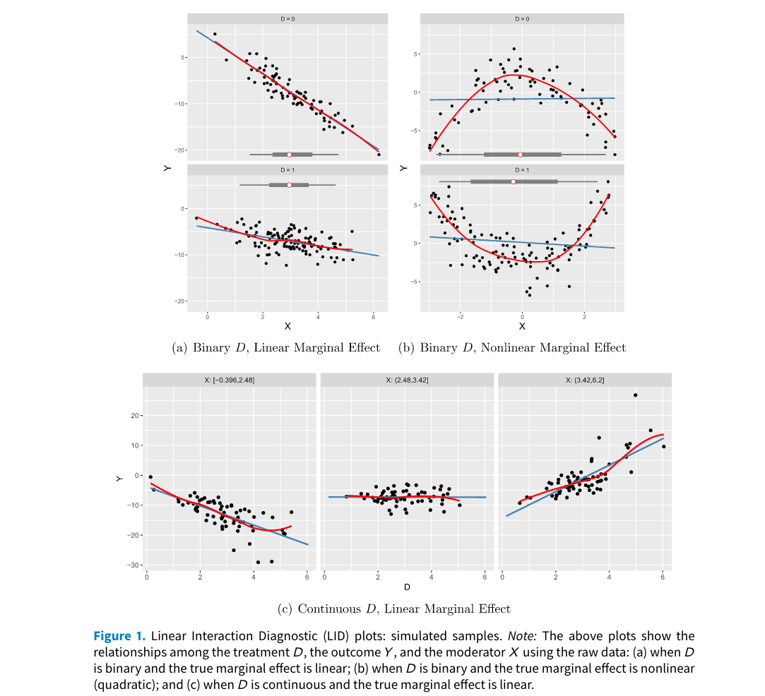
• Diagnostic Tool To asses the validity or invalidity of LIE and common support assumptions, they suggest usage of Linear-Interaction-Diagnostic (LID plots).

Checking, if the linear regression lines (blue) and the LOESS fits (red) diverge considerably across the range of X values, and compare the distribution of X in both groups and examine the range of X values for which there are a sufficient number of data points for the estimation of marginal effects. Taken from Page 169 in Hainmueller, J., Mummolo, J., & Xu, Y. (2019). How Much Should We Trust Estimates from Multiplicative Interaction Models? Simple Tools to Improve Empirical Practice. Political Analysis, 27(2), 163–192. https://doi.org/10.1017/pan.2018.46

Estimation- They propose two alternative estimation strategies:

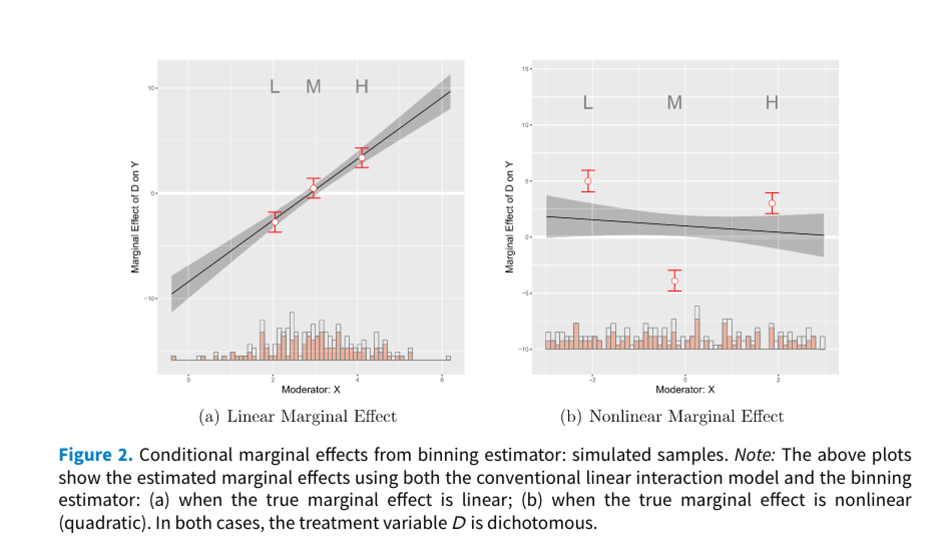
• Binning estimator: This approach discretizes the moderator into bins and allows for different treatment effects in each bin, capturing non-linearity. As the authors state, “the binning estimator is much more flexible as it jointly fits the interaction components of the standard model to each bin separately, thereby relaxing the LIE assumption” (p. 177).

\[ Y = \sum_{j=1}^{3} \big\{\mu_j + \alpha_j D + \eta_j (X - x_j) + \beta_j (X - x_j)D\big\} G_j + Z\gamma + \epsilon \]

where, \(G_js\) are dummy variables for bins. When entire range is split into three bins according to treciles. They are defined as shown below,

\[ G_1 = \begin{cases} 1 & X < \delta_{1/3}, \\ 0 & \text{otherwise}, \end{cases} \quad G_2 = \begin{cases} 1 & X \in [\delta_{1/3}, \delta_{2/3}], \\ 0 & \text{otherwise}, \end{cases} \quad G_3 = \begin{cases} 1 & X \geq \delta_{2/3}, \\ 0 & \text{otherwise}. \end{cases} \]

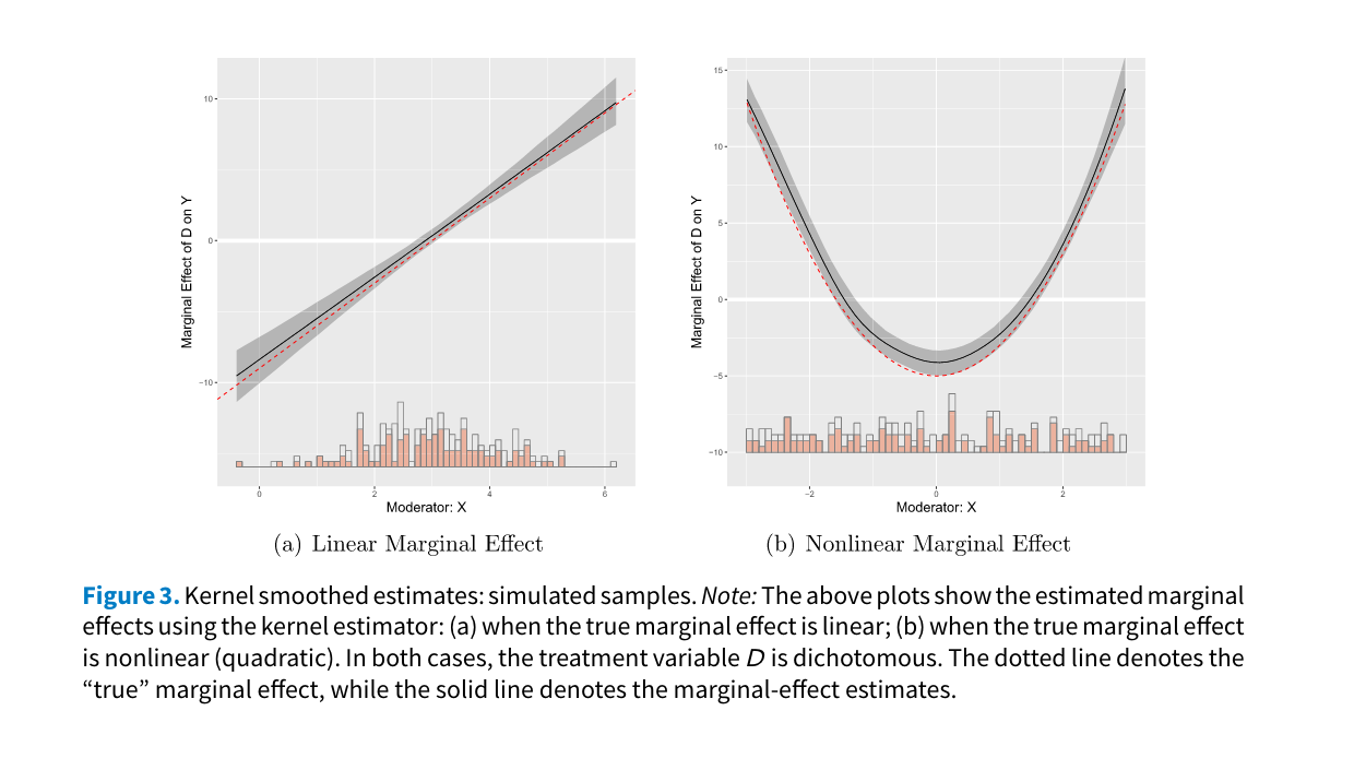
• Kernel estimator: This method employs non-parametric smoothing to estimate the conditional marginal effect of the treatment across the range of the moderator, again relaxing the LIE assumption. The output is a smooth function rather than a set of discrete point estimates, making it potentially less straightforward to summarize and interpret compared to the binning estimator ¹.

Moderation using interflex package

The solutions discussed above are incorporated by Jens Hainmueller, Jiehan Liu, Licheng Liu, Ziyi Liu, Jonathan Mummolo, Tianzhu Qin, and Yiqing Xu in interflex package. The functions in it estimates, interprets, and visualizes marginal effects and performs diagnostics, as proposed by Hainmueller, Mummolo, and Xu (2019) ².

# Load package
# install.packages("interflex")
library(interflex)

# Comes with simulated datasets
# Code on construction of simulation datasets is given below
# No need to run. It is just for reference
data(interflex)
ls()

[1] "s1" "s2" "s3" "s4" "s5" "s6" "s7" "s8" "s9"

set.seed(1234)
n<-200
d1<-sample(c(0,1),n,replace=TRUE) # dichotomous treatment
d2<-rnorm(n,3,1) # continuous treatment
x<-rnorm(n,3,1) # moderator
z<-rnorm(n,3,1) # covariate
e<-rnorm(n,0,1) # error term

## linear marginal effect
y1<-5 - 4 * x - 9 * d1 + 3 * x * d1 + 1 * z + 2 * e
y2<-5 - 4 * x - 9 * d2 + 3 * x * d2 + 1 * z + 2 * e
s1<-cbind.data.frame(Y = y1, D = d1, X = x, Z1 = z)
s2<-cbind.data.frame(Y = y2, D = d2, X = x, Z1 = z)

## quadratic marginal effect
x3 <- runif(n, -3,3) # uniformly distributed moderator
y3 <- d1*(x3^2-2.5) + (1-d1)*(-1*x3^2+2.5) + 1 * z + 2 * e
s3 <- cbind.data.frame(D=d1, X=x3, Y=y3, Z1 = z)

## adding two-way fixed effects
n  <- 500
d4 <-sample(c(0,1),n,replace=TRUE) # dichotomous treatment
x4 <- runif(n, -3,3) # uniformly distributed moderator
z4 <- rnorm(n, 3,1) # covariate
alpha <- 20 * rep(rnorm(n/10), each = 10)
xi <- rep(rnorm(10), n/10)
y4 <- d4*(x4^2-2.5) + (1-d4)*(-1*x4^2+2.5) + 1 * z4 + alpha + xi + 
  2 * rnorm(n,0,1)
s4 <- cbind.data.frame(D=d4, X=x4, Y=y4, Z1 = z4, 
                       unit = rep(1:(n/10), each = 10),
                       year = rep(1:10, (n/10)))

## Multiple treatment arms
n <- 600
# treatment 1
d1 <- sample(c('A','B','C'),n,replace=T)
# moderator
x <- runif(n,min=-3, max = 3)
# covriates
z1 <- rnorm(n,0,3)
z2 <- rnorm(n,0,2)
# error
e <- rnorm(n,0,1)
y1 <- rep(NA,n)
y1[which(d1=='A')] <- -x[which(d1=='A')]
y1[which(d1=='B')] <- (1+x)[which(d1=='B')]
y1[which(d1=='C')] <- (4-x*x-x)[which(d1=='C')]
y1 <- y1 + e + z1 + z2
s5 <- cbind.data.frame(D=d1, X=x, Y=y1, Z1 = z1,Z2 = z2)

s1 is a case of a dichotomous treatment indicator with linear marginal effects;
s2 is a case of a continuous treatment indicator with linear marginal effects;
s3 is a case of a dichotomous treatment indicator with nonlinear marginal effects;
s4 is a case of a dichotomous treatment indicator, nonlinear marginal effects, with additive two-way fixed effects; and

s5 is a case of a discrete treatment indicator, nonlinear marginal effects, with additive two-way fixed effects.

Raw LID Plots

Let’s check different types of datsets and outputs

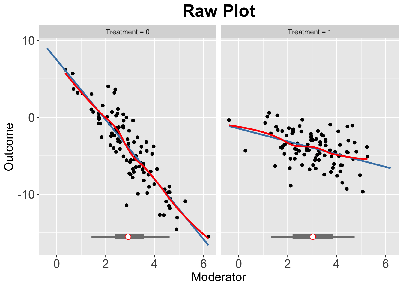
1. Dichotomous treatment indicator with linear marginal effects.

interflex(estimator = "raw",
          Y = "Y", 
          D = "D", 
          X = "X", 
          data = s1, 
          weights = NULL,
          Ylabel = "Outcome", Dlabel = "Treatment", Xlabel="Moderator", 
          main = "Raw Plot", cex.main = 1.2, ncols=2
          )

Baseline group not specified; choose treat = 0 as the baseline group. 

2. Continuous treatment indicator with linear marginal effects.
   

interflex(estimator = "raw", Y = "Y", D = "D", X = "X", data = s2,
          Ylabel = "Outcome", Dlabel = "Treatment", Xlabel="Moderator", 
          theme.bw = TRUE, show.grid = FALSE, ncols=3)

3. Dichotomous treatment indicator with nonlinear marginal effects.

interflex(estimator = "raw", Y = "Y", D = "D", X = "X", data = s3,
          Ylabel = "Outcome", Dlabel = "Treatment", 
          Xlabel="Moderator",ncols=3)

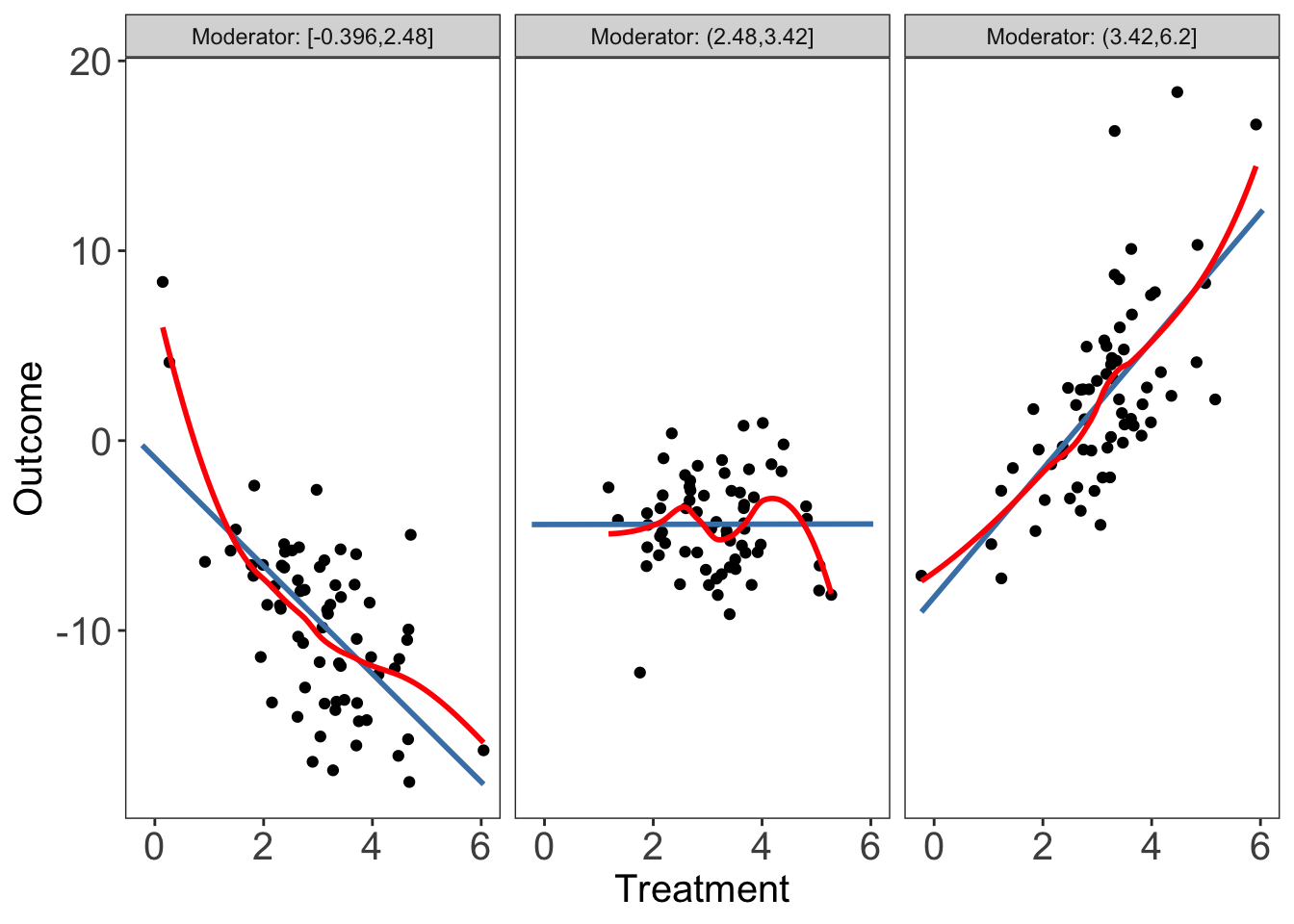
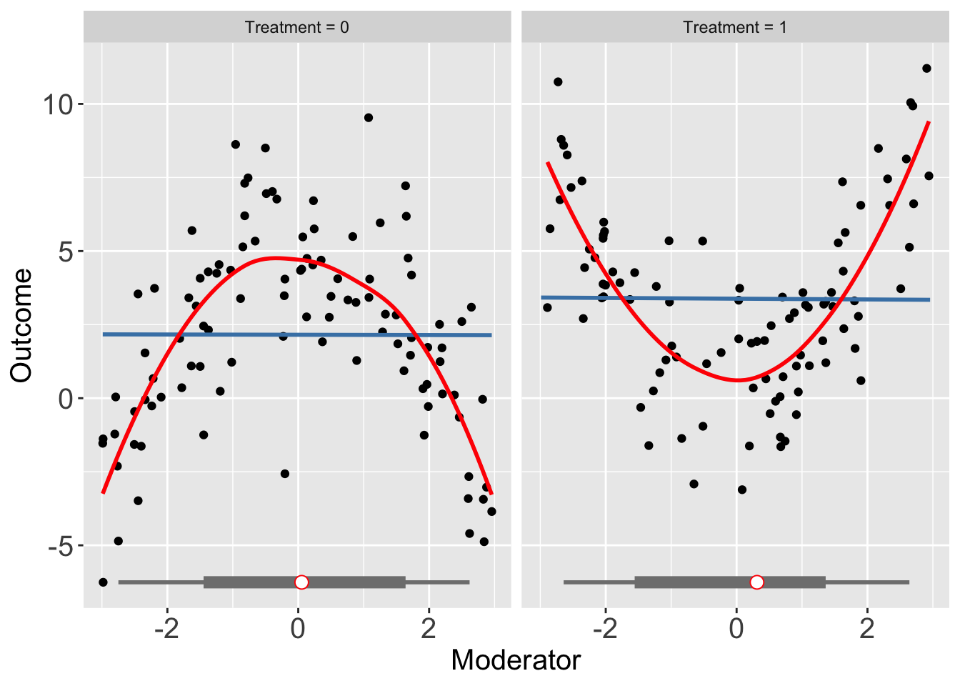
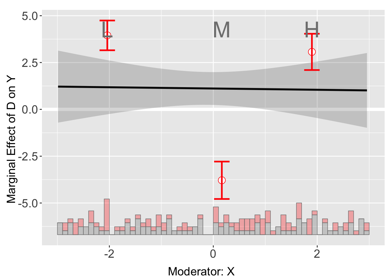
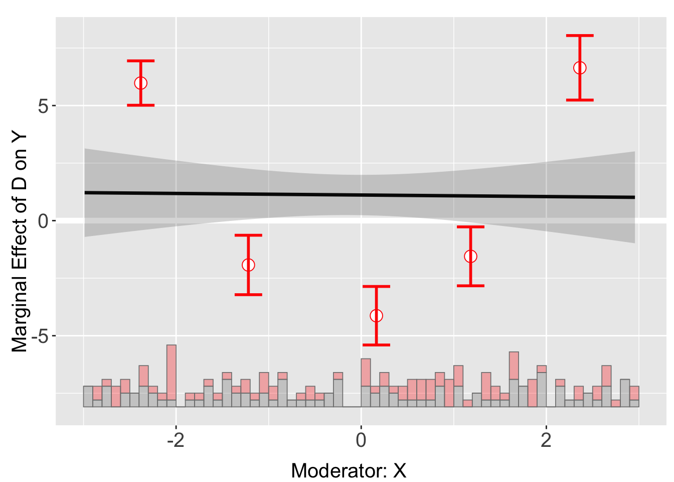
Baseline group not specified; choose treat = 0 as the baseline group. 

Interpretation Exercise

1. Interpret the three plots. What do the red and blue lines signify?

2. In which of them LIE seems to be violated?

3. Which seems to be suffering from lack of common support?

Read the documentation with ?interflex and 3. Diagnostics section in Hainmueller, Mummolo, and Xu (2019).

Binning Estimator

We will use s1 dataset. The data generating process underlying it is

\[ Y = -5 - 4X - 9D + 3X \times D + Z + 2\epsilon \]

out <- interflex(Y = "Y", D = "D", X = "X", Z = "Z1", data = s1, 
                 estimator = "binning", vcov.type = "robust", 
                 main = "Marginal Effects", ylim = c(-15, 15))

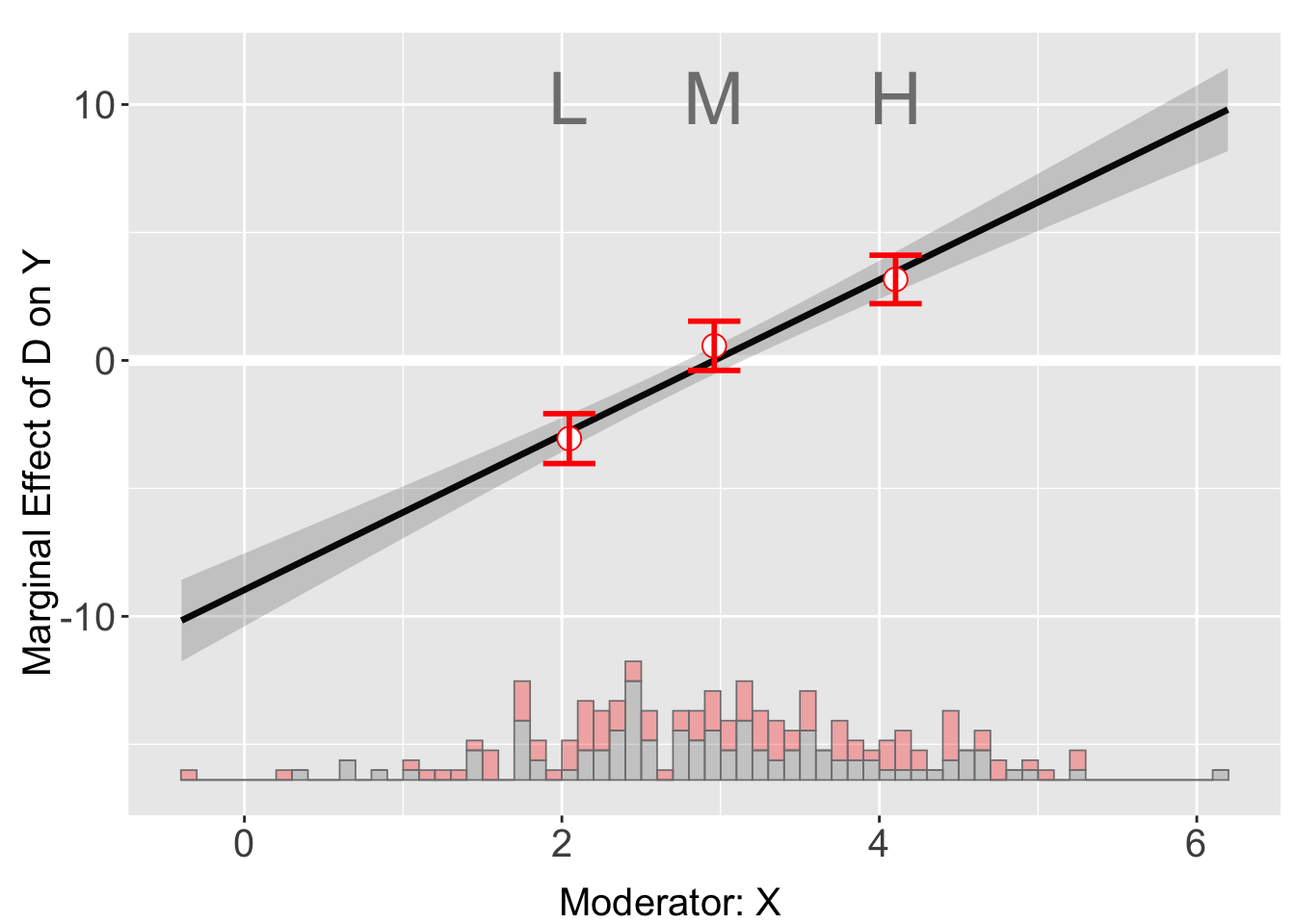
Baseline group not specified; choose treat = 0 as the baseline group. 

plot(out)

How are the bins created in this plot?

Also, interpret the histogram at the bottom.

Note that interflex will also automatically report a set of statistics when estimator = “binning”, including: (1) the binning estimates and their standard errors and 95% confidence intervals, (2) the percentage of observations within each bin, (3) the L-kurtosis of the moderator, and (4) a Wald test to formally test if we can reject the linear multiplicative interaction model by comparing it with a more flexible model of multiple bins

print(out$tests$p.wald)

[1] "0.526"

Interpreting the wald test p-vlue We see that the Wald test cannot reject the NULL hypothesis that the linear interaction model and the three-bin model are statistically equivalent.

When LIE is not valid

Let’s look at dataset s3, which is simulated from the following data generating process,

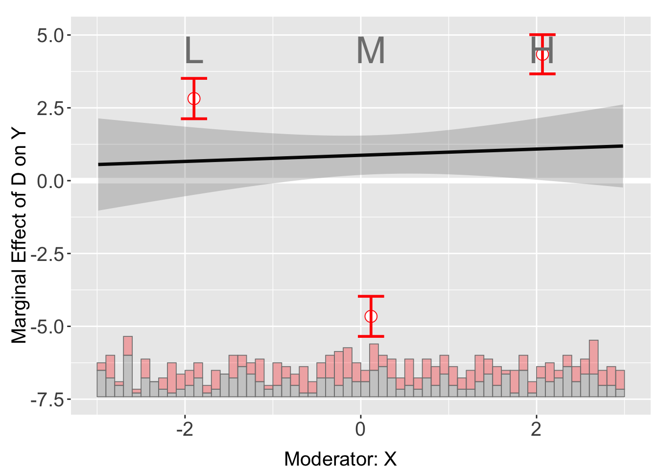
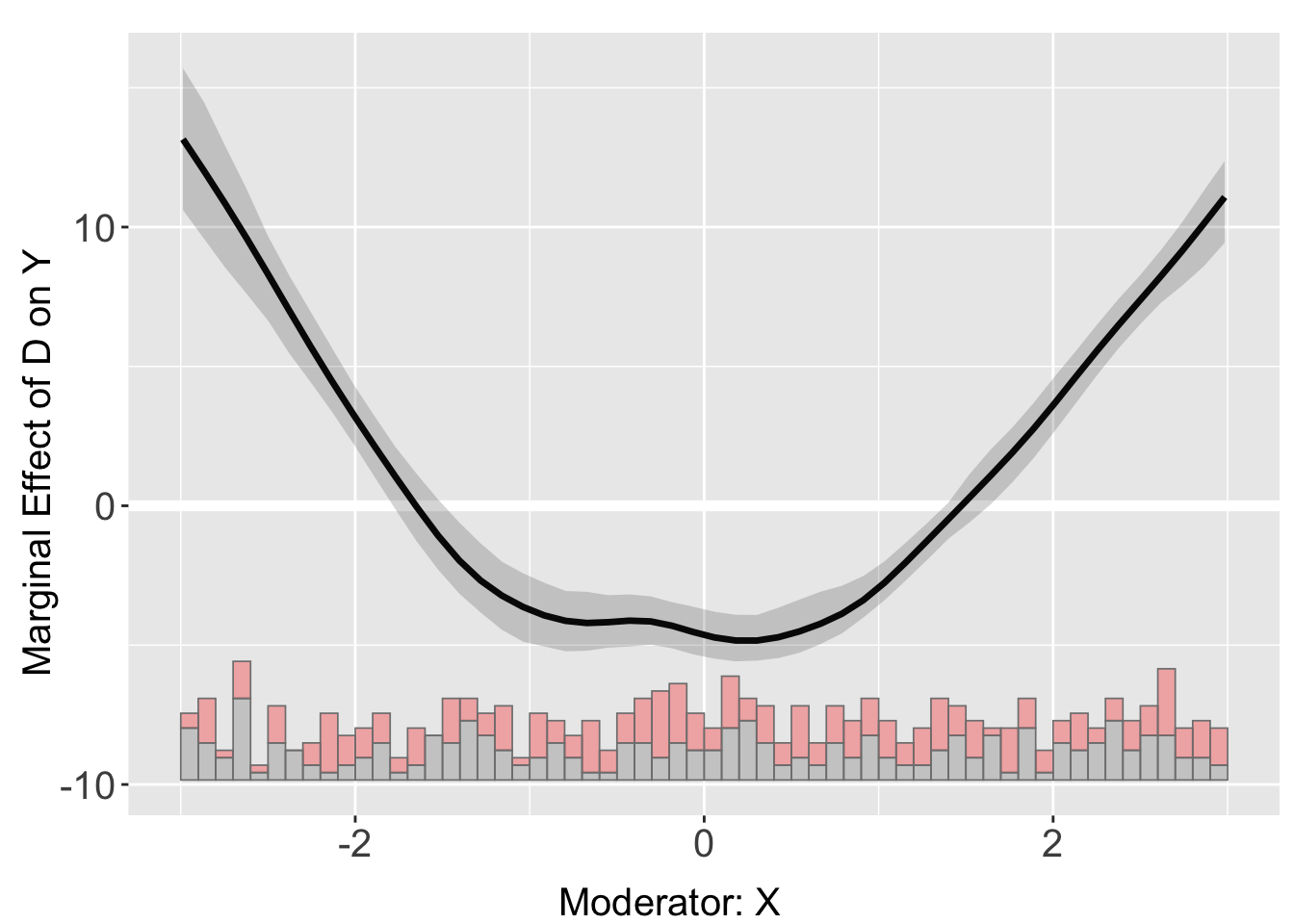
\[ Y = 2.5 - 2.5D - X^2 + 2(D \times X^2) + Z + \varepsilon \] The marginal effect of D on Y is

\[ \frac{\partial Y}{\partial D} = -2.5 + 2X^2 \] which is non-linear interaction. However, by estimating with linear interaction assumption, we would have missed out this facet and get biased results.

out_li <- interflex(Y = "Y", D = "D", X = "X", Z = "Z1", data = s3, 
                    estimator = "linear") 

Baseline group not specified; choose treat = 0 as the baseline group. 

plot(out_li)

Binning estimator gives a better insight into the non-linear interactive relationship.

out_nli <- interflex(Y = "Y", D = "D", X = "X", Z = "Z1", data = s3, 
                     estimator = "binning")

Baseline group not specified; choose treat = 0 as the baseline group. 

plot(out_nli)

Let’s increase the number of bins.

out_nli_5 <- interflex(Y = "Y", D = "D", X = "X", Z = "Z1", 
                       data = s3, nbins = 5,
                     estimator = "binning", main = "With 5 bins")

Baseline group not specified; choose treat = 0 as the baseline group. 

plot(out_nli_5)

Conducting wald tests again, for the new models with 3 and 5 bins.

print(out_nli$tests$p.wald)

[1] "0.000"

print(out_nli_5$tests$p.wald)

[1] "0.000"

This time the NULL hypothesis that the linear interaction model and the three-bin model are statistically equivalent is safely rejected (p.wald = 0.00).

Kernel Estimator

Imagine, increasing the number of bins infinitely. We would be somewhat capturing the underlying relationship, in a smoothed curve ³.

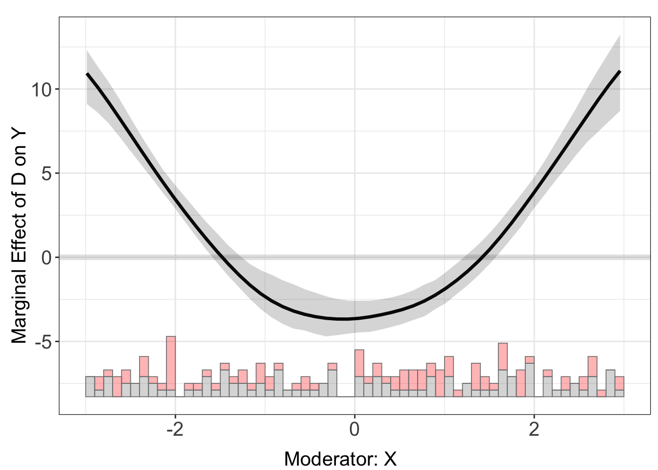
The kernel estimator is a method used to flexibly estimate the functional form of a marginal effect across the values of a moderator variable, relaxing the linear interaction effect (LIE) assumption and offering protection against the problem of lack of common support.

out_ke <- interflex(Y = "Y", D = "D", X = "X", Z = "Z1", data = s3, 
                 estimator = "kernel", theme.bw = TRUE)

Baseline group not specified; choose treat = 0 as the baseline group. 
Cross-validating bandwidth ... 
Parallel computing with 4 cores...
Optimal bw=0.5244.
Number of evaluation points:50
Parallel computing with 4 cores...

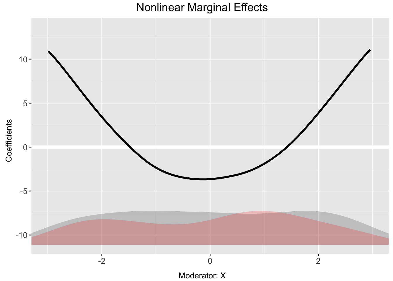
out_ke$figure

Note

You can change the plotting attributes, without running the interflex function again. See code below how it uses same out_ke output from interflex function inside a plotting command

plot(out_ke, main = "Nonlinear Marginal Effects",
     ylab = "Coefficients",
     Xdistr = "density", # Instead of histogram, density curve
     xlim = c(-3,3), ylim = c(-10,12),
     CI = FALSE, cex.main = 0.8, cex.lab = 0.7, cex.axis = 0.7) 

The semi-parametric marginal effect estimates are stored in out$est.kernel.

Note that we can use the file option to save a plot to a file in interflex (e.g. by setting file = "myplot.pdf" or file = "myplot.png").

Features of Kernel Estimator

Advantages:

Flexibility: Allows the conditional effect of the treatment variable to vary freely across the range of the moderator, capturing nonlinear and nonmonotonic relationships4.

Protection against extrapolation: Estimates the marginal effect across the full range of the moderator, highlighting areas with limited common support through wider confidence intervals57.

Automated bandwidth selection: The bandwidth parameter, h, which determines the smoothness of the estimated function, is automatically selected through cross-validation, minimizing subjectivity8.

Limitation

The output is a smooth function rather than a set of discrete point estimates, making it potentially less straightforward to summarize and interpret compared to the binning estimator

Estimation with Fixed effects

Focusing on dataset s4, which has the following DGP

\[ Y = \beta_0 + \beta_1 D + \beta_2 X^2 + \beta_3 (D \times X^2) + \beta_4 Z + \alpha + \xi + \varepsilon \]

The regression includes both unit fixed effects (\(\alpha\)) and year fixed effects (\(\xi\)), which control for unobserved heterogeneity across units (such as individuals or firms) and years (such as time effects).

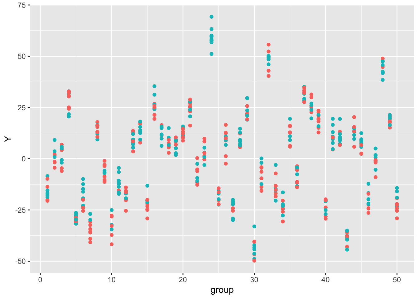
Remember in s4, a large chunk of the variation in the outcome variable is driven by group fixed effects (see the code where simulated datasets are created above). Below is a scatterplot of the raw data (group index vs. outcome). Red and green dots represent treatment and control units, respectively. We can see that outcomes are highly correlated within a group.

ggplot(s4, aes(x=group, y = Y, colour = as.factor(D))) + geom_point() + guides(colour=FALSE) 

Warning: The `<scale>` argument of `guides()` cannot be `FALSE`. Use "none" instead as
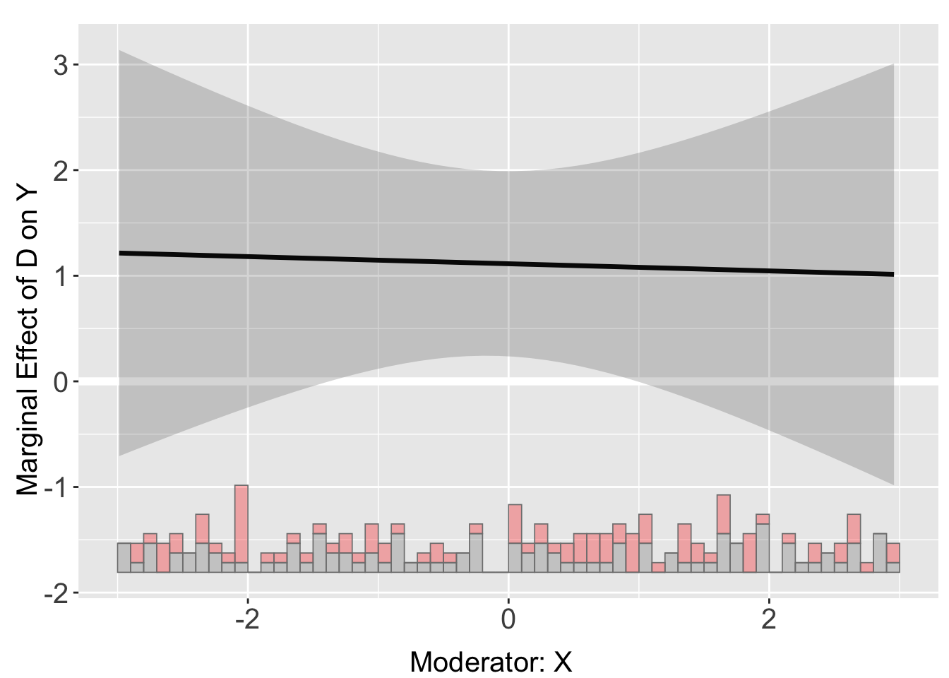
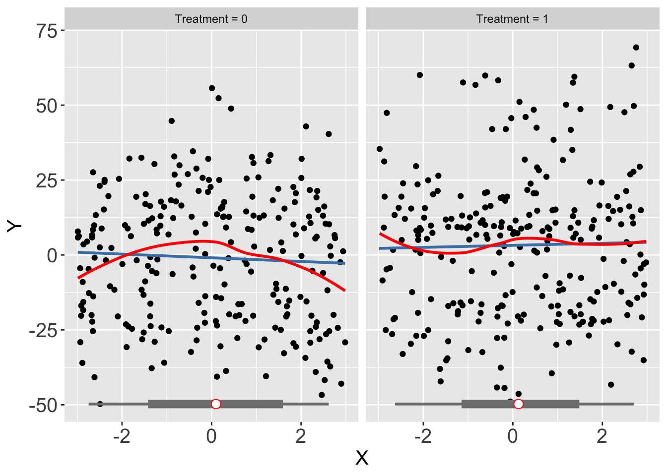
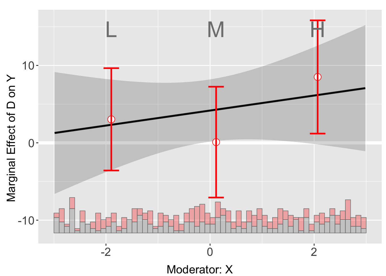
of ggplot2 3.3.4.

When fixed effects are present, it is possible that we cannot observe a clear pattern of marginal effects in the raw plot as before, while binning estimates have wide confidence intervals.

interflex(estimator = "raw", Y = "Y", D = "D", X = "X", 
          data = s4, weights = NULL,ncols=2)

Baseline group not specified; choose treat = 0 as the baseline group. 

# binning
s4.binning <- interflex(Y = "Y", D = "D", X = "X", Z = "Z1", 
                        data = s4, estimator = "binning",
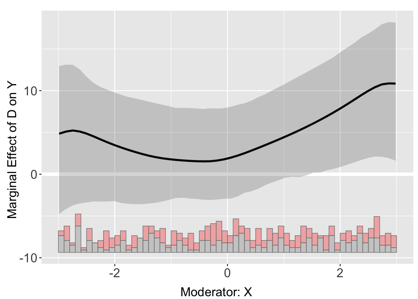
                        FE = NULL, cl = "group")

Baseline group not specified; choose treat = 0 as the baseline group. 

plot(s4.binning)

Similarly, kernel estimates have wide cross-validated bandwidths.

# Kernel
s4$wgt <- 1
s4.kernel <- interflex(Y = "Y", D = "D", X = "X", Z = "Z1",
                       data = s4, estimator = "kernel",
                       FE = NULL, cl = "group", weights = "wgt")

Baseline group not specified; choose treat = 0 as the baseline group. 
Cross-validating bandwidth ... 
Parallel computing with 4 cores...
Optimal bw=1.3539.
Number of evaluation points:50
Parallel computing with 4 cores...

plot(s4.kernel)

The issues are caused by in-correct identification and specification of the model.

The binning and kernel estimates are much more informative when fixed effects are included, by using the FE option. Note that the number of group indicators can exceed 2. The algorithm is optimized for a large number of fixed effects or many group indicators. The cl option controls the level at which standard errors are clustered.

Binning with FE

s4.binning <- interflex(Y = "Y", D = "D", X = "X", Z = "Z1", 
                        data = s4, estimator = "binning", 
                        FE = c("group", "year"), cl = "group", 
                        weights = "wgt")

Baseline group not specified; choose treat = 0 as the baseline group. 

plot(s4.binning)

Kernel with FE

s4.kernel <- interflex(Y = "Y", D = "D", X = "X", Z = "Z1", 
                       data = s4, estimator = "kernel",
                       FE = c("group","year"), cl = "group")

Baseline group not specified; choose treat = 0 as the baseline group. 
Cross-validating bandwidth ... 
Parallel computing with 4 cores...
Optimal bw=0.3514.
Number of evaluation points:50
Parallel computing with 4 cores...

plot(s4.kernel)

Visualizing Heterogeneity in Effect

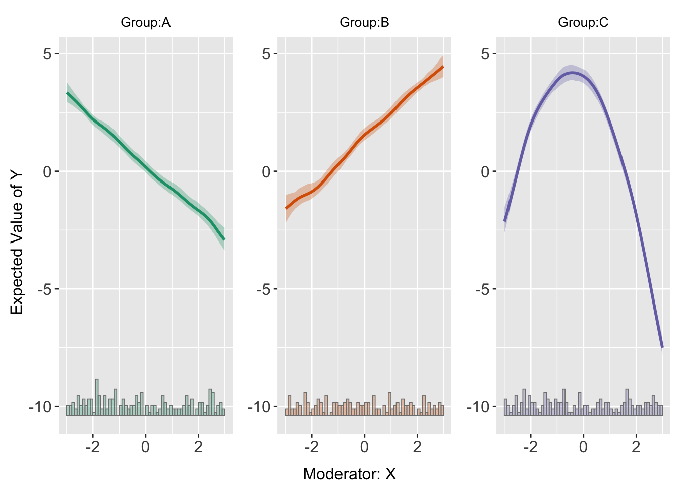
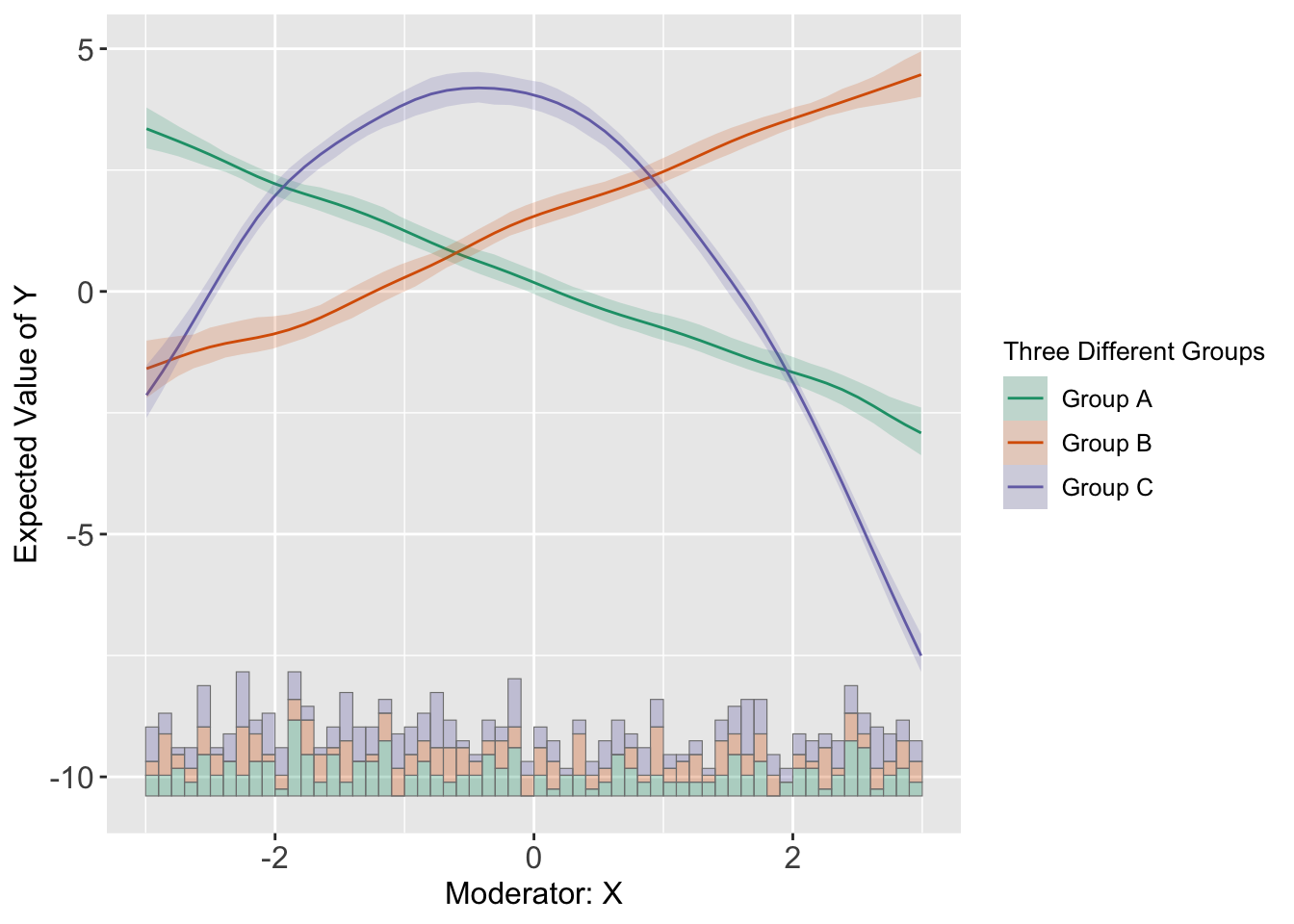
We can use interflex to visualize predicted outcomes based on non-linear interaction that we just analysed.

s5.kernel <-interflex(Y = "Y", D = "D", X = "X", Z = c("Z1", "Z2"),
                      data = s5, estimator = "kernel")

Baseline group not specified; choose treat = A as the baseline group. 
Cross-validating bandwidth ... 
Parallel computing with 4 cores...
Optimal bw=0.3522.
Number of evaluation points:50
Parallel computing with 4 cores...

predict(s5.kernel)

Or, by setting pool = TRUE,

predict(s5.kernel,order = c('A','B','C'),
        subtitle = c("Group A", "Group B", "Group C"), pool = T,
        legend.title = "Three Different Groups")

Additional Notes on Advanced Issues

The documentation of the interflex package also has examples of application to cases of Multiple (>2) Treatment Arms, as well as analysing Difference in Treatment Effects at Different Values of the Moderator.

The interflex function also incorporate the interaction terms between the moderator X and all covariates Z in models to reduce biases induced by their correlations (Blackwell and Olson 2022). Though not recommended, users can turn off this option by setting full.moderate = FALSE.

While Hainmueller, Mummolo, and Xu (2019) provide much needed disgnostics and estimation tools, Beiser-McGrath and Beiser-McGrath (2023) argue that by allowing simply for non-linear interaction between treatment and moderator, “researchers can infer nonlinear interaction effects, even though the true interaction effect is linear, when variables used for covariate adjustment that are correlated with the moderator have a nonlinear effect upon the outcome of interest”. If the research includes moderated effects, the latter paper is recommended to be read.

In-class Exercise

Use the replication dataset that you have been using till now to perform the following:

1. Identify a covariate that could plausibly be driving heterogeneity in treatment effect. You could use theoretical priors or your experience of working with this dataset to inform your choice.

2. Write down two versions of possible moderation in the data generating process - linear and non-linear interaction ones.

3. Make LID plots to assess your hypothesised interactions in 2.

4. Use interflex function to assess moderation with binning as well as kernel estimators.

5. Use wald-test p-value from interflex output to comment on your inference.

Beiser-McGrath, Janina, and Liam F. Beiser-McGrath. 2023. “The Consequences of Model Misspecification for the Estimation of Nonlinear Interaction Effects.” Political Analysis 31 (2): 278–87. https://doi.org/10.1017/pan.2022.25.

Blackwell, Matthew, and Michael P. Olson. 2022. “Reducing Model Misspecification and Bias in the Estimation of Interactions.” Political Analysis 30 (4): 495–514. https://doi.org/10.1017/pan.2021.19.

Brambor, Thomas, William Roberts Clark, and Matt Golder. 2006. “Understanding Interaction Models: Improving Empirical Analyses.” Political Analysis 14 (1): 63–82. https://doi.org/10.1093/pan/mpi014.

Hainmueller, Jens, Jonathan Mummolo, and Yiqing Xu. 2019. “How Much Should We Trust Estimates from Multiplicative Interaction Models? Simple Tools to Improve Empirical Practice.” Political Analysis 27 (2): 163–92. https://doi.org/10.1017/pan.2018.46.

King, Gary, and Langche Zeng. 2006. “The Dangers of Extreme Counterfactuals.” Political Analysis 14 (2): 131–59. https://doi.org/10.1093/pan/mpj004.

---

1. The kernel estimator discussed in the Hainmueller paper is considered semi-parametric because it uses:
   A non-parametric approach: to estimate the potentially nonlinear relationship between the outcome, the treatment, and the moderator.
   A parametric approach: for the relationship between the outcome and the control variables.
   Also see, https://en.wikipedia.org/wiki/Kernel_density_estimation.

2. The code and discussion below has been adapted from the vignette of the package available at https://yiqingxu.org/packages/interflex/RGuide.html.

3. This is not fully what happens in kernel smoothening but is nevertheless a good learning/heuristic tool.