File Management and Workflow
Why Programming or Coding? (Revisiting)
Coding is about formalizing your thinking about how you treat the data and automating the formalization task to be done repetitively. It improves efficiency, enhances reproducibility, and boosts creativity when it comes to finding new patterns in your data.
Benchmarks for reproducible data and statistical analyses:1
- Accuracy: Write a code that reduces the chances of making an error and lets you catch one if it occurs.
- Efficiency: If you are doing it twice, see the pattern of your decision-making and formalize it in your code. Difference between Excel and coding
- Replicate-and-Reproduce: Ability to repeat the computational process which reflects your thinking and decisions that you took along the way. Improves transparency and forces one to be deliberate and responsible about choices during analyses.
- Human Interpretability: Writing code is not just about analyzing but allowing yourself and then others to be able to understand your analytic choices.
- Public Good: Research is a public good. And the code allows your research to be truly accessible. This means you write a code that anyone else who understands the language can read, reuse, and recreate without you being present. We essentially ensure that by writing a readable and ideally publicly accessible code.
Guidelines
The article “Ten Simple Rules for Reproducible Computational Research” by Sandve et al. (2013) provides guidelines to ensure that computational research is reproducible, transparent, and robust. Here’s a summary of the key points:
| Rule | Description | Notes |
|---|---|---|
| Documentation | Track how results are produced, including all steps in the analysis workflow. | Keep short notes on reults |
| Automation | Minimize manual data manipulation by using scripts and documenting any manual changes. | Make changes to raw data in your scripts |
| Version Control | Use version control systems for all custom scripts to track changes and maintain reproducibility. | Using Github |
| Comprehensive Records | Archive all versions of external programs used, all intermediate results, and exact observation conditions. | Keep notes about data in comments |
| Accessibility | Make raw data, scripts, and results publicly accessible to enhance transparency and replication. | Maintainig good workflow |
File Management and Workflow
Understanding Absolute and Relative Paths
When working with files in any programming environment, paths specify the location of files and folders. These paths can be absolute or relative, and the choice between them significantly impacts reproducibility, portability, and ease of collaboration
Absolute Paths An absolute path provides the complete address of a file or folder, starting from the root directory of the file system. It tells the software exactly where to find a file, regardless of where the script is run.
Example: C:/Users/YourName/Documents/Project/Data/raw_data.dta
Relative Paths A relative path specifies the location of a file or folder relative to a “base directory” (e.g., the project’s working directory). It does not start from the root directory but instead is calculated based on the location of the script.
Suppose your working directory is set to: C:/Users/YourName/Documents/Project
Then, a relative path might look like: Data/raw_data.dta
Key Differences Between Absolute and Relative Paths
| Feature | Absolute Path | Relative Path |
|---|---|---|
| Starting Point | Starts from the root directory of the file system. | Starts from the current working directory. |
| Portability | Not portable—specific to the user’s system. | Highly portable—adapts to different systems. |
| Ease of Sharing | Harder to share; others must update paths. | Easier to share; no changes needed if structure is consistent. |
| Use Case | Best for fixed environments or one-off scripts. | Ideal for collaborative and reproducible projects. |
| Flexibility | Breaks if the file is moved or the system changes. | Adapts as long as the folder structure remains consistent. |
R Projects
We used the setwd() command till now to trace the files we need in our work. As your work expands, projects will have multiple datasets to be loaded, different subsidiary scripts to be used, and multiple outputs to be saved.
A first order problem related to both file management and reproducibility of code is the usage of file paths. Using absolute paths, like ~/User/MyName/Documents/..... becomes cumbersome and also inhibits efficiency of reproducibility. Every time someone else runs the script, they will have to change the file paths in all the instances in Rscripts or .qmd file to locate the related datasets as well as other objects. Similarly, there would be issues with saving objects in new places. A partially efficient way we used till now involved using setwd() to direct R to a new working directory; this is also called usage of relative paths
R Projects is a built-in mechanism in RStudio for seamless file management and usage of relative paths.
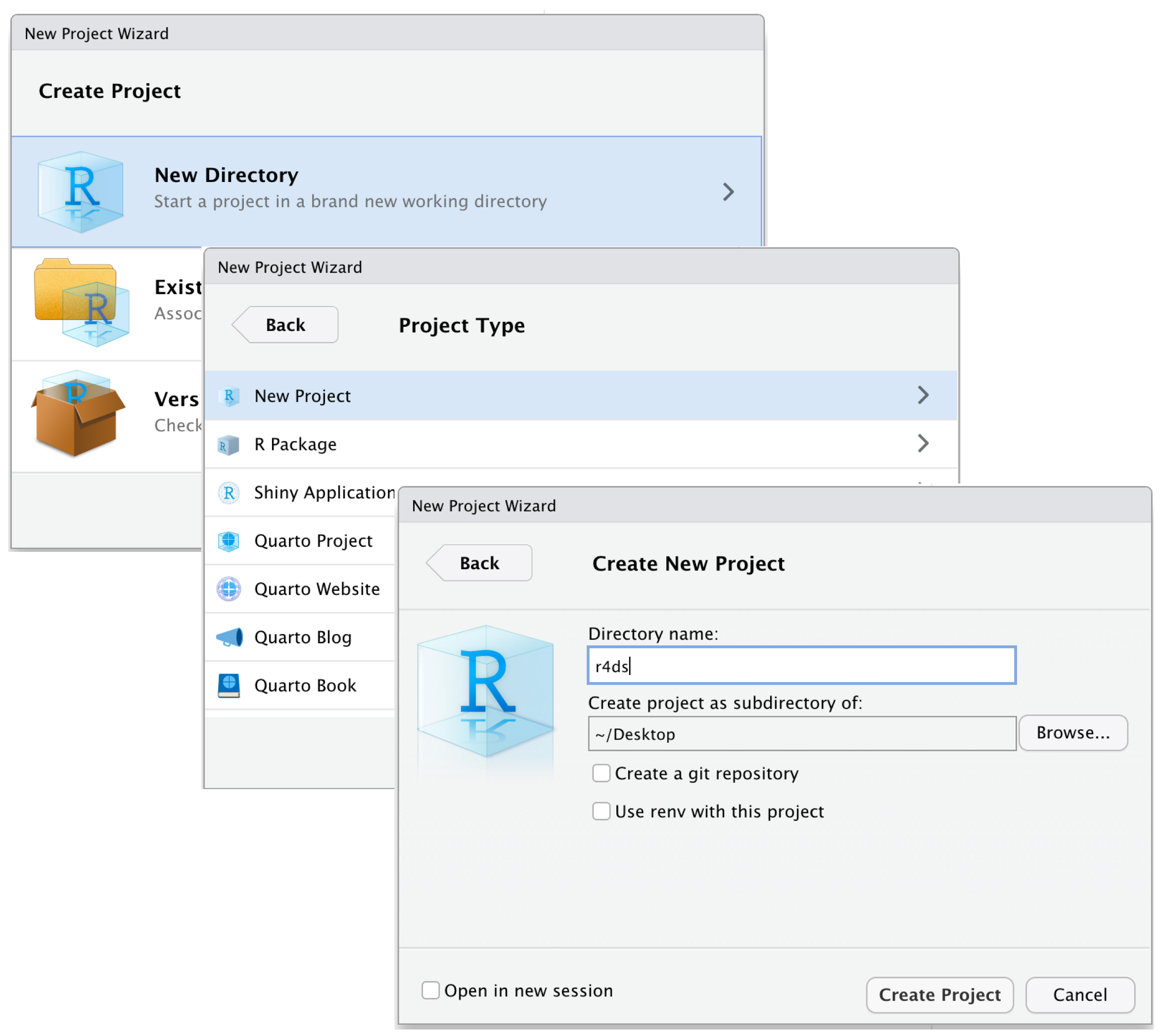
Let’s start by creating a new project. Click File > New Project. Name the new project govt-8001-dataessay.
Standardized Folder and File Structure (here package)
An efficient file and folder management system is going to be crucial as we move into working with serious projects. Storing using all the files associated with a project in a comprehensible folder system is facilitated in both R and Stata. You would ideally want to create your own template for folder management that you follow across projects.
An efficient file and folder management system is going to be crucial as we move into working with serious projects. As stressed earlier, keeping and using all the files associated with a project in a comprehensible folder system is facilitated by R Projects. You would ideally want to create your own template for folder management that you follow across proejcts. For starters, the folder structure below is the one created for your data essay assignment in Govt 8001 or Quant 1.
You can use the point-and-click fucntionality in your computers to create this structure. Later today, we will briefly go through an R script that do this programmatically.
📦 govt-8001-dataessay
├─ govt-8001-dataessay.RProj
├─ 000-setup.R
├─ 001-eda.qmd
├─ 002-analysis.qmd
└─ 003-manuscript.qmd
├─ Data
│  ├─ Raw
│  │  ├─ Dataset1
│  │  │  ├─ dataset1.csv
│  │  │  └─ codebook-dataset1.pdf
│  │  └─ Dataset2
│  │     ├─ ...dta
│  │     └─ codebook-dataset2.pdf
│  └─ Clean
│     └─ Merged-df1-df2.csv
├─ Scripts
│  ├─ R-scripts
│  │  ├─ plotting-some-variable.R
│  │  └─ exploring-different-models.R
│  ├─ Stata-Scripts
│  │  └─ seeing-variable-labels.do
│  └─ Python-Scripts
│     └─ scraping-data-from-website.py
└─ Outputs
   ├─ Plots
   │  ├─ ...jpeg
   │  └─ ...png
   ├─ Tables
   │  └─ .csv
   └─ Text
      └─ ...txt
Suggested folder structure for a Quant-1 project
While we learnt how to create or associate an .RProj with a folder, integrating it with here() function from the here package, makes workflow smoother. Let’s do it with the following exercise.
Make it a habit of using R Projects and here() function in your scripts for writing portable code.
You can read this quick and informative blogpost on using these two here.
Takeaways
Here’s a quick workflow for starting a new project or assignment or paper.
Make a new folder in your computer with apt name. Ideally,
govt-<coursecode>-<project>.Start RStudio.
Create a new Rstudio Project by clicking
File > New Project. Name itgovt-<coursecode>-<project.Check if now your RStudio Window shows the project name on top right corner. If not, go to folder and double-click the
.RProjfile.Paste the
000-setup.Rfile in the main project folder. Open it in the same Rstudio window with the project and run the complete file. Your folder structure is created.Copy your raw data in
Data/Rawfolder. Similarly, your scripts inScripts/RScriptsfolderStart your new
.qmdfile and save it in the main folder.Remember to use
here()package extensively in both, scripts and quarto files, when loading or saving the data.You can zip the whole project folder for sharing. The receiver will just need to unzip and run the code after starting the associated
.RProjfile, without changing file paths on their computer.
Inspired by the summary provided by Prof Aaron Williams’ course on Data Analysis offered at McCourt School. Strongly recommended to learn good coding using R↩︎